
Power Series Solutions
A power series solution writes y = Σ aₙxⁿ and finds the coefficients from the differential equation. Substitute the series into the equation, shift indices so every term has xⁿ, and set each coefficient to 0. That gives a recurrence relation for the coefficients, which builds the solution from a₀ = y(0) and a₁ = y′(0).
Before this lesson: Power Series, Differentiating and Integrating Power Series and Second-Order Homogeneous Linear Equations
Why use power series?
The characteristic equation solves y″ + by′ + cy = 0 only when b and c are constants. Many important equations have coefficients that change with x, such as Airy’s equation y″ − xy = 0. Their solutions are usually not elementary functions, but they can still be written as power series.
The idea is to treat the unknown coefficients a₀, a₁, a₂, … like unknown numbers. The equation must hold for every x, so the coefficient of each power of x must be 0. That turns one differential equation into infinitely many simple algebra equations.
Ordinary points and the main theorem
Write the equation as P(x)y″ + Q(x)y′ + R(x)y = 0 with polynomial coefficients. A point x₀ is an ordinary point if P(x₀) ≠ 0. Otherwise it is a singular point, and you need the Method of Frobenius instead.
Theorem: near an ordinary point x₀, the equation has two independent solutions of the form y = Σ aₙ(x − x₀)ⁿ. Each series converges at least for |x − x₀| < ρ, where ρ is the distance from x₀ to the nearest zero of P, counting complex zeros.
Term-by-term differentiation gives the series for y′ and y″:
y = \sum_{n=0}^{\infty} a_nx^n,\qquad y' = \sum_{n=1}^{\infty} na_nx^{n-1},\qquad y'' = \sum_{n=2}^{\infty} n(n-1)a_nx^{n-2}How to find a power series solution
- Write y, y′ and y″ as the series above.
- Substitute them into the equation, multiplying any powers of x into the sums.
- Shift each index so every sum has xⁿ, and note where each sum starts.
- Set the coefficient of each xⁿ equal to 0. Handle any starting terms (like n = 0) on their own, then solve the general equation for the highest coefficient. This is the recurrence relation.
- Compute the coefficients from a₀ and a₁ and write the solution, grouping the a₀ terms and the a₁ terms.
Power series solutions examples
Example 1: A familiar equation
Find the power series solution of y″ + y = 0 about x = 0.
y'' = \sum_{n=2}^{\infty} n(n-1)a_nx^{n-2}Differentiate y = Σ aₙxⁿ twice (differentiating power series).
\sum_{n=2}^{\infty} n(n-1)a_nx^{n-2} = \sum_{n=0}^{\infty} (n+2)(n+1)a_{n+2}x^nReplace n by n + 2 so the power is xⁿ (sigma notation index shift).
\sum_{n=0}^{\infty} \left[(n+2)(n+1)a_{n+2} + a_n\right]x^n = 0Substitute into y″ + y = 0 and combine the sums.
(n+2)(n+1)a_{n+2} + a_n = 0Every coefficient of a zero power series is 0.
a_{n+2} = -\dfrac{a_n}{(n+2)(n+1)}Solve for aₙ₊₂: the recurrence relation.
a_2 = -\dfrac{a_0}{2},\quad a_4 = -\dfrac{a_2}{12} = \dfrac{a_0}{24}Use n = 0, then n = 2.
a_3 = -\dfrac{a_1}{6},\quad a_5 = -\dfrac{a_3}{20} = \dfrac{a_1}{120}Use n = 1, then n = 3.
y = a_0\left(1 - \dfrac{x^2}{2!} + \dfrac{x^4}{4!} - \cdots\right) + a_1\left(x - \dfrac{x^3}{3!} + \dfrac{x^5}{5!} - \cdots\right)Group the even and odd terms.
y = a_0\cos x + a_1\sin x
Recognize the Maclaurin series of cos x and sin x.
Answer: y = a₀ cos x + a₁ sin x, the same answer the characteristic equation gives in complex roots of the characteristic equation. The method works; the next examples use it where the characteristic equation cannot.
Example 2: Airy’s equation
Find the first three nonzero terms of each of the two independent solutions of y″ − xy = 0 about x = 0.
xy = \sum_{n=0}^{\infty} a_nx^{n+1} = \sum_{n=1}^{\infty} a_{n-1}x^nMultiply y by x, then replace n by n − 1.
\sum_{n=0}^{\infty} (n+2)(n+1)a_{n+2}x^n - \sum_{n=1}^{\infty} a_{n-1}x^n = 0Substitute y″ (shifted as in Example 1) and xy.
2a_2 = 0 \Rightarrow a_2 = 0
The x⁰ term appears only in the first sum.
(n+2)(n+1)a_{n+2} - a_{n-1} = 0,\quad n \ge 1Match the coefficients of xⁿ for n ≥ 1.
a_{n+2} = \dfrac{a_{n-1}}{(n+2)(n+1)}Solve; each coefficient comes from the one three places back.
a_3 = \dfrac{a_0}{6},\quad a_6 = \dfrac{a_3}{30} = \dfrac{a_0}{180}Use n = 1, then n = 4.
a_4 = \dfrac{a_1}{12},\quad a_7 = \dfrac{a_4}{42} = \dfrac{a_1}{504}Use n = 2, then n = 5.
a_5 = \dfrac{a_2}{20} = 0Use n = 3; a₂, a₅, a₈, … are all 0.
y = a_0\left(1 + \dfrac{x^3}{6} + \dfrac{x^6}{180} + \cdots\right) + a_1\left(x + \dfrac{x^4}{12} + \dfrac{x^7}{504} + \cdots\right)Group the a₀ terms and the a₁ terms.
Answer: y₁ = 1 + x³/6 + x⁶/180 + ⋯ and y₂ = x + x⁴/12 + x⁷/504 + ⋯. The leading coefficient P(x) = 1 is never 0, so both series converge for every x.
Example 3: A series that stops
Solve y″ − 2xy′ + 4y = 0 with y(0) = 1 and y′(0) = 0.
xy' = \sum_{n=0}^{\infty} na_nx^nMultiply y′ by x; the n = 0 term is 0, so the sum can start at n = 0.
\sum_{n=0}^{\infty} \left[(n+2)(n+1)a_{n+2} - 2na_n + 4a_n\right]x^n = 0Substitute; all three sums start at n = 0.
a_{n+2} = \dfrac{(2n - 4)a_n}{(n+2)(n+1)}Set each coefficient to 0 and solve for aₙ₊₂.
a_0 = 1,\quad a_1 = 0
a₀ = y(0) and a₁ = y′(0).
a_2 = \dfrac{(-4)(1)}{2} = -2Use n = 0.
a_4 = \dfrac{(0)(-2)}{12} = 0Use n = 2; 2n − 4 = 0, so every later even coefficient is 0 too.
a_3 = a_5 = a_7 = \cdots = 0
The odd coefficients are multiples of a₁ = 0.
y = 1 - 2x^2
Only a₀ and a₂ are left.
Answer: y = 1 − 2x². Check: y″ = −4, −2x(−4x) = 8x² and 4y = 4 − 8x², which add to 0. When the recurrence has a factor that becomes 0, the series stops and the solution is a polynomial.
Example 4: Recognizing the sum
Solve y″ + xy′ + y = 0 with y(0) = 1 and y′(0) = 0, find the sum of the series, and use the terms through x⁶ to estimate y(0.5).
\sum_{n=0}^{\infty} \left[(n+2)(n+1)a_{n+2} + na_n + a_n\right]x^n = 0Substitute the series for y″, xy′ and y.
(n+2)(n+1)a_{n+2} = -(n+1)a_nSet the coefficient to 0 and combine naₙ + aₙ.
a_{n+2} = -\dfrac{a_n}{n+2}Divide both sides by (n + 2)(n + 1).
a_2 = -\dfrac{1}{2},\quad a_4 = -\dfrac{a_2}{4} = \dfrac{1}{8},\quad a_6 = -\dfrac{a_4}{6} = -\dfrac{1}{48}Start from a₀ = 1; the odd coefficients are 0 because a₁ = 0.
y = 1 - \dfrac{x^2}{2} + \dfrac{x^4}{8} - \dfrac{x^6}{48} + \cdotsWrite the series.
y = e^{-x^2/2}Compare with eᵘ = 1 + u + u²/2! + u³/3! + ⋯ with u = −x²/2.
y(0.5) \approx 1 - 0.125 + 0.0078125 - 0.0003255 = 0.882487
Substitute x = 0.5 into the four terms.
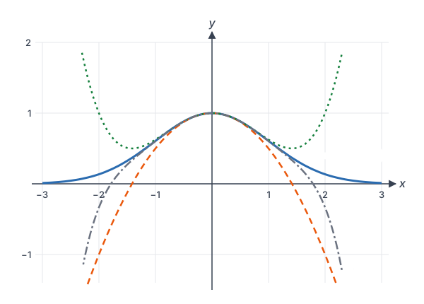
Answer: y = e^(−x²/2), and the four terms give y(0.5) ≈ 0.88249, while e^(−0.125) ≈ 0.88250. The graph shows the partial sums matching the solution near x = 0 and pulling away farther out.
Example 5: A spring that stiffens (word problem)
A mass on a spring that slowly stiffens follows y″ + ty = 0, with t in seconds and y in centimeters. It starts at y(0) = 1 with y′(0) = 0. Use the first three nonzero terms of the series to estimate y(1), and bound the error.
a_2 = 0,\quad a_{n+2} = -\dfrac{a_{n-1}}{(n+2)(n+1)}Same steps as Example 2, with +ty in place of −xy.
a_0 = 1,\quad a_1 = 0
Use the initial conditions, so the a₁ and a₂ chains are all 0.
a_3 = -\dfrac{a_0}{6} = -\dfrac{1}{6}Use n = 1.
a_6 = -\dfrac{a_3}{30} = \dfrac{1}{180}Use n = 4.
a_9 = -\dfrac{a_6}{72} = -\dfrac{1}{12960}Use n = 7; this is the first term left out.
y \approx 1 - \dfrac{t^3}{6} + \dfrac{t^6}{180}Keep the first three nonzero terms.
y(1) \approx 1 - 0.16667 + 0.00556 = 0.83889
Substitute t = 1.
Answer: y(1) ≈ 0.839 cm. At t = 1 the terms alternate in sign and shrink, so by the alternating series error bound the error is less than the first omitted term, 1/12960 ≈ 0.0000772. A numerical solver gives y(1) ≈ 0.83881.
Common mistakes
| Mistake | Example of the error | Fix |
|---|---|---|
| Shifting the power but not the starting index | Writing Σ from n = 2 of (n + 2)(n + 1)aₙ₊₂xⁿ | When n becomes n + 2, the start 2 becomes 0. |
| Combining sums that start at different n | Adding the Airy sums from n = 0 and n = 1 into one recurrence for all n | Treat the n = 0 term on its own: 2a₂ = 0. |
| Forgetting the factor from the shift | Writing aₙ₊₂ = −aₙ for y″ + y = 0 | The y″ coefficient is (n + 2)(n + 1)aₙ₊₂. |
| Mixing up the arbitrary constants | Using a₀ = y′(0) | a₀ = y(0) and a₁ = y′(0). |
| Assuming every series converges for all x | Claiming the solution of (1 + x²)y″ + y = 0 converges at x = 3 | P has zeros at ±i, so the guaranteed radius is only 1. |
| Expanding about a singular point | Using y = Σ aₙxⁿ for x²y″ + y = 0 | P(0) = 0, so x = 0 is singular; use the Method of Frobenius. |
Related ideas
Series about other points
To expand about x₀ ≠ 0, substitute t = x − x₀ so the new equation is centered at t = 0, then use the same method. The radius of convergence is measured from x₀, as in interval of convergence.
Special functions
Many named functions began as series solutions: Airy functions from Example 2, Hermite polynomials from equations like Example 3, and Legendre polynomials from (1 − x²)y″ − 2xy′ + k(k + 1)y = 0. Their properties are studied directly from the recurrence relation.
Practice problems
- Rewrite Σ from n = 2 to ∞ of n(n − 1)aₙxⁿ⁻² so that it has xⁿ and starts at n = 0.
- Find the recurrence relation and the general solution of y″ − y = 0 as power series.
- Solve y′ − y = 0 with a power series.
- Solve y″ + 4y = 0 with y(0) = 1 and y′(0) = 0 through the x⁶ term.
- For Airy’s equation y″ − xy = 0 with y(0) = 0 and y′(0) = 1, find the first three nonzero terms.
- Is x = 0 an ordinary point of (x − 2)y″ + y′ + y = 0? What radius of convergence is guaranteed?
- What radius of convergence is guaranteed for series solutions of (1 + x²)y″ + y = 0 about x = 0?
- Solve y″ − 2xy′ + 6y = 0 with y(0) = 0 and y′(0) = 1.
- Solve y″ + xy′ + y = 0 with y(0) = 0 and y′(0) = 1 through the x⁷ term.
- Use the first three nonzero terms of y₁ from Example 2 to estimate y₁(0.5).
Show answers
1.
m = n - 2 \Rightarrow n = m + 2
Let the new index be m; n = 2 becomes m = 0.
\sum_{m=0}^{\infty} (m+2)(m+1)a_{m+2}x^mSubstitute n = m + 2 everywhere.
Answer: Σ from n = 0 to ∞ of (n + 2)(n + 1)aₙ₊₂xⁿ, after renaming m as n
2.
(n+2)(n+1)a_{n+2} - a_n = 0Substitute and set each coefficient to 0.
a_{n+2} = \dfrac{a_n}{(n+2)(n+1)}Solve for aₙ₊₂.
a_{2k} = \dfrac{a_0}{(2k)!},\quad a_{2k+1} = \dfrac{a_1}{(2k+1)!}Apply the recurrence repeatedly.
Answer: y = a₀(1 + x²/2! + x⁴/4! + ⋯) + a₁(x + x³/3! + ⋯) = a₀ cosh x + a₁ sinh x (hyperbolic functions)
3.
\sum_{n=0}^{\infty} \left[(n+1)a_{n+1} - a_n\right]x^n = 0Shift y′ = Σ naₙxⁿ⁻¹ to start at n = 0 and subtract y.
a_{n+1} = \dfrac{a_n}{n+1} \Rightarrow a_n = \dfrac{a_0}{n!}Solve and apply repeatedly.
Answer: y = a₀(1 + x + x²/2! + ⋯) = a₀eˣ
4.
a_{n+2} = -\dfrac{4a_n}{(n+2)(n+1)}Recurrence from (n + 2)(n + 1)aₙ₊₂ + 4aₙ = 0.
a_2 = -\dfrac{4}{2} = -2,\quad a_4 = -\dfrac{4(-2)}{12} = \dfrac{2}{3}Use n = 0 and n = 2 with a₀ = 1.
a_6 = -\dfrac{4(2/3)}{30} = -\dfrac{4}{45}Use n = 4; the odd terms are 0 because a₁ = 0.
Answer: y = 1 − 2x² + (2/3)x⁴ − (4/45)x⁶ + ⋯, which is the series for cos 2x
5.
a_1 = 1,\quad a_0 = a_2 = 0
Initial conditions and 2a₂ = 0.
a_4 = \dfrac{a_1}{12} = \dfrac{1}{12},\quad a_7 = \dfrac{a_4}{42} = \dfrac{1}{504}Recurrence aₙ₊₂ = aₙ₋₁/((n + 2)(n + 1)) with n = 2 and n = 5.
Answer: y = x + x⁴/12 + x⁷/504 + ⋯
6.
P(0) = 0 - 2 = -2 \ne 0
Evaluate the coefficient of y″ at x = 0.
P(x) = 0 \Rightarrow x = 2
The nearest singular point.
Answer: yes, x = 0 is an ordinary point; the series converge at least for |x| < 2
7.
1 + x^2 = 0 \Rightarrow x = \pm i
Find the zeros of P, including complex ones.
|i - 0| = 1
Distance from 0 to ±i in the complex plane.
Answer: at least |x| < 1
8.
a_{n+2} = \dfrac{(2n - 6)a_n}{(n+2)(n+1)}Same steps as Example 3 with 6y.
a_3 = \dfrac{(2 - 6)(1)}{6} = -\dfrac{2}{3}Use n = 1 with a₁ = 1.
a_5 = \dfrac{(6 - 6)a_3}{20} = 0Use n = 3; the odd series stops. The even terms are 0 because a₀ = 0.
Answer: y = x − (2/3)x³
9.
a_{n+2} = -\dfrac{a_n}{n+2}Recurrence from Example 4.
a_3 = -\dfrac{1}{3},\quad a_5 = \dfrac{1}{15},\quad a_7 = -\dfrac{1}{105}Use n = 1, 3, 5 with a₁ = 1; a₅ = −a₃/5 and a₇ = −a₅/7.
Answer: y = x − x³/3 + x⁵/15 − x⁷/105 + ⋯
10.
y_1 \approx 1 + \dfrac{x^3}{6} + \dfrac{x^6}{180}First three nonzero terms from Example 2.
y_1(0.5) \approx 1 + 0.0208333 + 0.0000868 = 1.0209201
Substitute: 0.125/6 and 0.015625/180.
Answer: y₁(0.5) ≈ 1.02092
Power series solutions FAQ
What is an ordinary point of a differential equation?
For P(x)y″ + Q(x)y′ + R(x)y = 0 with polynomial coefficients, x₀ is an ordinary point if P(x₀) ≠ 0. Near an ordinary point, two independent power series solutions always exist.
How do you find the recurrence relation?
Substitute the series for y, y′ and y″, shift indices so every sum has xⁿ, and set the total coefficient of xⁿ equal to 0. Solving that equation for the highest-index coefficient gives the recurrence relation.
Why are a₀ and a₁ arbitrary?
Setting x = 0 in the series gives y(0) = a₀ and y′(0) = a₁. A second-order equation has two arbitrary constants, and these are the two; the recurrence fixes every other coefficient.
Where does a power series solution converge?
At least within distance ρ of the center, where ρ is the distance to the nearest zero of P(x), complex zeros included. If P is a nonzero constant, the series converge for every x.
Summary
- Near an ordinary point (P(x₀) ≠ 0), write y = Σ aₙxⁿ and substitute.
- Shift indices so every term has xⁿ, handle the starting terms, and set each coefficient to 0.
- The recurrence relation gives every coefficient from a₀ = y(0) and a₁ = y′(0).
- Group the a₀ terms and a₁ terms to get two independent solutions; sometimes a series stops and gives a polynomial.
- The series converge at least out to the nearest zero of P, complex zeros included.
Previous lesson: Nonlinear Systems and Stability
Next lesson: Method of Frobenius
Back to the Differential Equations Index