
Solving Linear Systems with Eigenvalues
To solve a linear system x′ = Ax whose matrix has real, different eigenvalues, find each eigenvalue λ of A and an eigenvector v for it. Each pair gives a solution e^(λt)v, and the general solution adds them: x = c₁e^(λ₁t)v₁ + c₂e^(λ₂t)v₂. Initial values then fix the constants.
Before this lesson: Systems of Differential Equations, Eigenvalues and Eigenvectors and Characteristic Polynomial
Why eigenvectors solve x′ = Ax
For one equation y′ = ay, the solution is y = Ce^(at). For a system, try the same shape: x = e^(λt)v, where λ is a number and v is a constant vector. The function e^(λt) only rescales v, so this solution moves along a straight line through the origin.
\mathbf{x}' = \lambda e^{\lambda t}\mathbf{v}Differentiate x = e^(λt)v; v is constant.
A\mathbf{x} = e^{\lambda t}A\mathbf{v}Multiply A by x; e^(λt) is a scalar.
\lambda e^{\lambda t}\mathbf{v} = e^{\lambda t}A\mathbf{v} \iff A\mathbf{v} = \lambda\mathbf{v}Set x′ = Ax and divide by e^(λt), which is never 0.
So x = e^(λt)v solves x′ = Ax exactly when v is an eigenvector of A with eigenvalue λ. A straight-line solution like this grows along v if λ is positive, shrinks toward the origin if λ is negative, and stays put if λ = 0.
The eigenvalue method for real, different eigenvalues
When an n × n matrix A has n different real eigenvalues, their eigenvectors are linearly independent, so the n straight-line solutions form a fundamental set. Every solution is a combination of them.
\mathbf{x}(t) = c_1e^{\lambda_1 t}\mathbf{v}_1 + c_2e^{\lambda_2 t}\mathbf{v}_2 + \cdots + c_ne^{\lambda_n t}\mathbf{v}_nHow to solve x′ = Ax with eigenvalues
- Find the eigenvalues: solve det(A − λI) = 0.
- For each eigenvalue λ, find an eigenvector v by solving (A − λI)v = 0.
- Write the general solution x = c₁e^(λ₁t)v₁ + c₂e^(λ₂t)v₂ + ….
- For an initial-value problem, set t = 0 and solve c₁v₁ + c₂v₂ + … = x(0) for the constants.
Any nonzero multiple of an eigenvector works. A different choice of v only changes the constants, not the solution.
Solving linear systems with eigenvalues: examples
Example 1: A general solution
Find the general solution of x′ = Ax with A = [1 2; 3 2].
\det(A - \lambda I) = (1 - \lambda)(2 - \lambda) - 2\cdot 3
Write the characteristic polynomial of a 2 × 2 matrix.
(1 - \lambda)(2 - \lambda) - 6 = \lambda^2 - 3\lambda + 2 - 6
Multiply out (1 − λ)(2 − λ).
\lambda^2 - 3\lambda - 4 = (\lambda - 4)(\lambda + 1)
Combine like terms and factor (see factoring trinomials).
\lambda_1 = 4,\quad \lambda_2 = -1
Set each factor equal to 0.
A - 4I = \begin{bmatrix} -3 & 2 \\ 3 & -2 \end{bmatrix} \Rightarrow -3v_1 + 2v_2 = 0Subtract 4 from each diagonal entry; the rows are multiples, so one equation remains.
\mathbf{v}_1 = \begin{bmatrix} 2 \\ 3 \end{bmatrix}Choose v₁ = 2, so v₂ = 3 (see eigenvalues and eigenvectors).
A + I = \begin{bmatrix} 2 & 2 \\ 3 & 3 \end{bmatrix} \Rightarrow v_1 + v_2 = 0Add 1 to each diagonal entry for λ = −1.
\mathbf{v}_2 = \begin{bmatrix} 1 \\ -1 \end{bmatrix}Choose v₁ = 1, so v₂ = −1.
\mathbf{x}(t) = c_1e^{4t}\begin{bmatrix} 2 \\ 3 \end{bmatrix} + c_2e^{-t}\begin{bmatrix} 1 \\ -1 \end{bmatrix}Combine the two straight-line solutions.
Answer: x(t) = c₁e^(4t)(2, 3) + c₂e^(−t)(1, −1). In components, x₁ = 2c₁e^(4t) + c₂e^(−t) and x₂ = 3c₁e^(4t) − c₂e^(−t). This matches the elimination answer in systems of differential equations, with much less algebra.
Example 2: An initial-value problem
Solve x′ = [−2 1; 1 −2]x with x(0) = (5, 1).
\det(A - \lambda I) = (-2 - \lambda)^2 - 1
Write the characteristic polynomial.
(-2 - \lambda)^2 - 1 = \lambda^2 + 4\lambda + 3
Expand and combine like terms.
\lambda^2 + 4\lambda + 3 = (\lambda + 1)(\lambda + 3)
Factor.
\lambda_1 = -1,\quad \lambda_2 = -3
Set each factor equal to 0.
A + I = \begin{bmatrix} -1 & 1 \\ 1 & -1 \end{bmatrix} \Rightarrow \mathbf{v}_1 = \begin{bmatrix} 1 \\ 1 \end{bmatrix}For λ = −1: −v₁ + v₂ = 0.
A + 3I = \begin{bmatrix} 1 & 1 \\ 1 & 1 \end{bmatrix} \Rightarrow \mathbf{v}_2 = \begin{bmatrix} 1 \\ -1 \end{bmatrix}For λ = −3: v₁ + v₂ = 0.
\mathbf{x}(t) = c_1e^{-t}\begin{bmatrix} 1 \\ 1 \end{bmatrix} + c_2e^{-3t}\begin{bmatrix} 1 \\ -1 \end{bmatrix}Write the general solution.
c_1 + c_2 = 5,\quad c_1 - c_2 = 1
Set t = 0 and match x(0) = (5, 1).
2c_1 = 6 \Rightarrow c_1 = 3
Add the equations (see elimination method) and divide by 2.
c_2 = 5 - 3 = 2
Substitute c₁ = 3 into c₁ + c₂ = 5.
x_1 = 3e^{-t} + 2e^{-3t},\quad x_2 = 3e^{-t} - 2e^{-3t}Substitute the constants and write each component.
Answer: x₁(t) = 3e^(−t) + 2e^(−3t) and x₂(t) = 3e^(−t) − 2e^(−3t). Both eigenvalues are negative, so every solution decays to the origin. The e^(−3t) part dies out faster, so for large t the solution comes in along the direction (1, 1).
Example 3: Eigenvalues of opposite signs
Solve x′ = [3 −2; 2 −2]x with x(0) = (1, −1), and describe the solution for large t.
\det(A - \lambda I) = (3 - \lambda)(-2 - \lambda) - (-2)(2)
Write the characteristic polynomial.
(3 - \lambda)(-2 - \lambda) + 4 = \lambda^2 - \lambda - 6 + 4
Multiply out the product.
\lambda^2 - \lambda - 2 = (\lambda - 2)(\lambda + 1)
Combine like terms and factor.
\lambda_1 = 2,\quad \lambda_2 = -1
Set each factor equal to 0.
A - 2I = \begin{bmatrix} 1 & -2 \\ 2 & -4 \end{bmatrix} \Rightarrow \mathbf{v}_1 = \begin{bmatrix} 2 \\ 1 \end{bmatrix}For λ = 2: v₁ − 2v₂ = 0.
A + I = \begin{bmatrix} 4 & -2 \\ 2 & -1 \end{bmatrix} \Rightarrow \mathbf{v}_2 = \begin{bmatrix} 1 \\ 2 \end{bmatrix}For λ = −1: 2v₁ − v₂ = 0.
2c_1 + c_2 = 1,\quad c_1 + 2c_2 = -1
Set t = 0 in c₁e^(2t)v₁ + c₂e^(−t)v₂ and match x(0).
c_2 = 1 - 2c_1
Solve the first equation for c₂.
c_1 + 2(1 - 2c_1) = -1
Substitute into the second equation (see substitution method).
-3c_1 + 2 = -1 \Rightarrow c_1 = 1
Distribute, combine like terms and solve.
c_2 = 1 - 2(1) = -1
Substitute c₁ = 1.
\mathbf{x}(t) = e^{2t}\begin{bmatrix} 2 \\ 1 \end{bmatrix} - e^{-t}\begin{bmatrix} 1 \\ 2 \end{bmatrix}Substitute the constants.
Answer: x₁(t) = 2e^(2t) − e^(−t) and x₂(t) = e^(2t) − 2e^(−t). As t grows, the e^(−t) part fades and the e^(2t) part takes over, so the solution heads off to infinity along the line through (2, 1). Only solutions that start exactly on the line through (1, 2) shrink to the origin. An equilibrium like this, with one growing and one shrinking direction, is called a saddle.
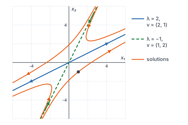
Example 4: Two tanks that trade water (word problem)
Two 50 L tanks are connected by two pipes. Water is pumped from tank 1 to tank 2 at 10 L/min and from tank 2 back to tank 1 at 10 L/min, so both volumes stay at 50 L. Tank 1 starts with 30 kg of salt and tank 2 with 10 kg. Find the salt amounts x₁(t) and x₂(t), and find when they differ by less than 1 kg.
x_1' = -\dfrac{10}{50}x_1 + \dfrac{10}{50}x_2 = -0.2x_1 + 0.2x_2Salt in from tank 2 minus salt out to tank 2, as in mixing problems.
x_2' = 0.2x_1 - 0.2x_2
Tank 2 gains what tank 1 loses.
\det(A - \lambda I) = (-0.2 - \lambda)^2 - 0.04 = \lambda^2 + 0.4\lambda
Write the characteristic polynomial and expand.
\lambda(\lambda + 0.4) = 0 \Rightarrow \lambda_1 = 0,\quad \lambda_2 = -0.4
Factor out λ.
\mathbf{v}_1 = \begin{bmatrix} 1 \\ 1 \end{bmatrix},\quad \mathbf{v}_2 = \begin{bmatrix} 1 \\ -1 \end{bmatrix}For λ = 0: −0.2v₁ + 0.2v₂ = 0; for λ = −0.4: 0.2v₁ + 0.2v₂ = 0.
\mathbf{x}(t) = c_1\begin{bmatrix} 1 \\ 1 \end{bmatrix} + c_2e^{-0.4t}\begin{bmatrix} 1 \\ -1 \end{bmatrix}Write the general solution; e^(0t) = 1.
c_1 + c_2 = 30,\quad c_1 - c_2 = 10
Match x(0) = (30, 10).
c_1 = 20,\quad c_2 = 10
Add the equations to get 2c₁ = 40, then substitute.
x_1 = 20 + 10e^{-0.4t},\quad x_2 = 20 - 10e^{-0.4t}Write each component.
x_1 - x_2 = 20e^{-0.4t} \lt 1Subtract the components and set the difference below 1.
e^{-0.4t} \lt 0.05Divide both sides by 20.
-0.4t \lt \ln 0.05
Take ln of both sides; ln is increasing (see solving exponential equations).
t \gt \dfrac{\ln 0.05}{-0.4} \approx 7.49Divide by −0.4 and reverse the inequality.
Answer: x₁(t) = 20 + 10e^(−0.4t) and x₂(t) = 20 − 10e^(−0.4t) kilograms. The amounts differ by less than 1 kg after about 7.49 minutes. The eigenvalue 0 gives the constant solution (20, 20), where the salt is split evenly; the total, x₁ + x₂ = 40 kg, never changes.
Example 5: A 3 × 3 system
Solve x′ = Ax with A = [1 0 0; 2 3 0; −1 1 −2] and x(0) = (3, 2, 0).
\lambda_1 = 1,\quad \lambda_2 = 3,\quad \lambda_3 = -2
A is triangular, so its eigenvalues are its diagonal entries.
(A - I)\mathbf{v} = \mathbf{0}:\ 2v_1 + 2v_2 = 0,\quad -v_1 + v_2 - 3v_3 = 0Subtract 1 from each diagonal entry; row 1 is all zeros.
v_2 = -v_1,\quad -2v_1 = 3v_3
Solve the first equation for v₂ and substitute into the second.
\mathbf{v}_1 = \begin{bmatrix} 3 \\ -3 \\ -2 \end{bmatrix}Choose v₁ = 3 to clear the fraction.
(A - 3I)\mathbf{v} = \mathbf{0}:\ -2v_1 = 0,\quad -v_1 + v_2 - 5v_3 = 0Subtract 3 from each diagonal entry; row 2 repeats row 1.
\mathbf{v}_2 = \begin{bmatrix} 0 \\ 5 \\ 1 \end{bmatrix}v₁ = 0 and v₂ = 5v₃; choose v₃ = 1.
(A + 2I)\mathbf{v} = \mathbf{0}:\ 3v_1 = 0,\quad 2v_1 + 5v_2 = 0Add 2 to each diagonal entry; the third row gives −v₁ + v₂ = 0.
\mathbf{v}_3 = \begin{bmatrix} 0 \\ 0 \\ 1 \end{bmatrix}v₁ = 0 and v₂ = 0, and v₃ is free.
3c_1 = 3,\quad -3c_1 + 5c_2 = 2,\quad -2c_1 + c_2 + c_3 = 0
Set t = 0 and match x(0) = (3, 2, 0).
c_1 = 1
Divide the first equation by 3.
-3 + 5c_2 = 2 \Rightarrow c_2 = 1
Substitute c₁ = 1 into the second equation and solve.
-2 + 1 + c_3 = 0 \Rightarrow c_3 = 1
Substitute c₁ and c₂ into the third equation and solve.
\mathbf{x}(t) = e^{t}\begin{bmatrix} 3 \\ -3 \\ -2 \end{bmatrix} + e^{3t}\begin{bmatrix} 0 \\ 5 \\ 1 \end{bmatrix} + e^{-2t}\begin{bmatrix} 0 \\ 0 \\ 1 \end{bmatrix}Substitute the constants.
Answer: x₁ = 3e^t, x₂ = −3e^t + 5e^(3t) and x₃ = −2e^t + e^(3t) + e^(−2t). Check with Av = λv: A(3, −3, −2) = (3, −3, −2), A(0, 5, 1) = (0, 15, 3) and A(0, 0, 1) = (0, 0, −2).
Common mistakes
| Mistake | Example of the error | Fix |
|---|---|---|
| Pairing an eigenvector with the wrong eigenvalue | x = c₁e^(4t)(1, −1) + c₂e^(−t)(2, 3) for A = [1 2; 3 2] | Check Av = λv for each pair: (2, 3) goes with 4 and (1, −1) with −1. |
| Leaving the vectors out | x = c₁e^(4t) + c₂e^(−t) | Each term is a scalar function times a vector: c₁e^(4t)(2, 3) + c₂e^(−t)(1, −1). |
| Subtracting λ from every entry | A − λI = [1 − λ 2 − λ; 3 − λ 2 − λ] | Subtract λ only on the main diagonal. |
| Not setting t = 0 in the exponentials | c₁e^4(2, 3) + c₂e^(−1)(1, −1) = x(0) | At t = 0 every e^(λt) equals 1: c₁(2, 3) + c₂(1, −1) = x(0). |
| Using the zero vector as an eigenvector | For λ = 4, taking v = (0, 0) | Eigenvectors are nonzero; pick a free variable value such as v₁ = 2. |
| Thinking a different eigenvector gives a wrong answer | Using (4, 6) instead of (2, 3) and calling the result different | Multiples of v only rescale c; the solution of an initial-value problem comes out the same. |
Related ideas
What the signs of the eigenvalues tell you
If every eigenvalue is negative, all solutions decay to the origin, as in Example 2. If every eigenvalue is positive, all solutions except x = 0 grow. If the signs differ, the origin is a saddle, as in Example 3. Phase Portraits draws and names all of these cases.
Diagonalization and decoupling
If P has the eigenvectors as columns and D has the eigenvalues on its diagonal, then A = PDP⁻¹ by diagonalization. Setting x = Py turns x′ = Ax into y′ = Dy, which is n separate equations yᵢ′ = λᵢyᵢ. The eigenvalue method is this change of variables written out.
Complex and repeated eigenvalues
If det(A − λI) = 0 has complex roots, the eigenvalue method still works, but you rewrite the solutions with sines and cosines; see Complex Eigenvalues. If a root repeats and there are not enough eigenvectors, you need an extra solution; see Repeated Eigenvalues.
Practice problems
- Find the general solution of x′ = [4 1; 2 3]x.
- Show that x = e^(3t)(1, 2) is a solution of x′ = [1 1; 4 1]x.
- Find the general solution of x′ = [1 1; 4 1]x.
- Solve the system in Problem 3 with x(0) = (0, 4).
- Solve x′ = [−5 2; 2 −2]x with x(0) = (4, 3).
- Describe the solution of Problem 5 as t → ∞.
- Write y″ − y′ − 6y = 0 as a first-order system, find the eigenvalues and eigenvectors of its matrix, and give y(t).
- Find the eigenvalues and eigenvectors of A = [2 1 0; 0 −1 1; 0 0 3] and write the general solution of x′ = Ax.
- A 100 L tank and a 50 L tank trade water at 10 L/min each way. All 15 kg of salt starts in the 50 L tank. Find the salt amounts x₁(t) (100 L tank) and x₂(t) (50 L tank).
- Solve x′ = [0 1; 1 0]x with x(0) = (2, 0).
Show answers
1.
\lambda^2 - 7\lambda + 10 = (\lambda - 2)(\lambda - 5)
det(A − λI) = (4 − λ)(3 − λ) − 2 = λ² − 7λ + 10; factor.
A - 5I = \begin{bmatrix} -1 & 1 \\ 2 & -2 \end{bmatrix} \Rightarrow \mathbf{v} = \begin{bmatrix} 1 \\ 1 \end{bmatrix}For λ = 5: −v₁ + v₂ = 0.
A - 2I = \begin{bmatrix} 2 & 1 \\ 2 & 1 \end{bmatrix} \Rightarrow \mathbf{v} = \begin{bmatrix} 1 \\ -2 \end{bmatrix}For λ = 2: 2v₁ + v₂ = 0.
Answer: x = c₁e^(5t)(1, 1) + c₂e^(2t)(1, −2)
2.
A\begin{bmatrix} 1 \\ 2 \end{bmatrix} = \begin{bmatrix} 1 + 2 \\ 4 + 2 \end{bmatrix} = \begin{bmatrix} 3 \\ 6 \end{bmatrix} = 3\begin{bmatrix} 1 \\ 2 \end{bmatrix}Multiply A by (1, 2) (see matrix multiplication).
Answer: (1, 2) is an eigenvector for λ = 3, so e^(3t)(1, 2) is a solution
3.
\lambda^2 - 2\lambda - 3 = (\lambda - 3)(\lambda + 1)
det(A − λI) = (1 − λ)² − 4; expand and factor.
A + I = \begin{bmatrix} 2 & 1 \\ 4 & 2 \end{bmatrix} \Rightarrow \mathbf{v} = \begin{bmatrix} 1 \\ -2 \end{bmatrix}For λ = −1: 2v₁ + v₂ = 0.
Answer: x = c₁e^(3t)(1, 2) + c₂e^(−t)(1, −2)
4.
c_1 + c_2 = 0,\quad 2c_1 - 2c_2 = 4
Set t = 0 and match x(0) = (0, 4).
c_2 = -c_1 \Rightarrow 4c_1 = 4 \Rightarrow c_1 = 1
Substitute c₂ = −c₁ into the second equation.
c_2 = -1
Use c₂ = −c₁.
Answer: x₁ = e^(3t) − e^(−t), x₂ = 2e^(3t) + 2e^(−t)
5.
\lambda^2 + 7\lambda + 6 = (\lambda + 1)(\lambda + 6)
det(A − λI) = (−5 − λ)(−2 − λ) − 4; expand and factor.
\mathbf{v}_1 = \begin{bmatrix} 1 \\ 2 \end{bmatrix},\quad \mathbf{v}_2 = \begin{bmatrix} 2 \\ -1 \end{bmatrix}For λ = −1: −4v₁ + 2v₂ = 0; for λ = −6: v₁ + 2v₂ = 0.
c_1 + 2c_2 = 4,\quad 2c_1 - c_2 = 3
Match x(0) = (4, 3).
c_1 = 4 - 2c_2 \Rightarrow 8 - 5c_2 = 3 \Rightarrow c_2 = 1
Substitute c₁ = 4 − 2c₂ into the second equation.
c_1 = 4 - 2 = 2
Substitute c₂ = 1.
Answer: x = 2e^(−t)(1, 2) + e^(−6t)(2, −1), so x₁ = 2e^(−t) + 2e^(−6t) and x₂ = 4e^(−t) − e^(−6t)
6.
e^{-6t} \text{ decays faster than } e^{-t}Compare the two terms.
Answer: the solution approaches the origin, coming in along the direction (1, 2) of the slower eigenvalue −1
7.
\mathbf{x}' = \begin{bmatrix} 0 & 1 \\ 6 & 1 \end{bmatrix}\mathbf{x}Let x₁ = y and x₂ = y′; then y″ = 6y + y′.
\lambda^2 - \lambda - 6 = (\lambda - 3)(\lambda + 2)
det(A − λI) = −λ(1 − λ) − 6; factor.
\mathbf{v}_1 = \begin{bmatrix} 1 \\ 3 \end{bmatrix},\quad \mathbf{v}_2 = \begin{bmatrix} 1 \\ -2 \end{bmatrix}The first row of A − λI gives −λv₁ + v₂ = 0, so v = (1, λ).
Answer: y = x₁ = c₁e^(3t) + c₂e^(−2t)
8.
\lambda = 2,\ -1,\ 3
A is triangular; read the diagonal.
(A - 2I)\mathbf{v} = \mathbf{0} \Rightarrow \mathbf{v} = (1, 0, 0)Rows give v₂ = 0 and then v₃ = 0.
(A + I)\mathbf{v} = \mathbf{0} \Rightarrow \mathbf{v} = (1, -3, 0)Rows give v₃ = 0 and 3v₁ + v₂ = 0.
(A - 3I)\mathbf{v} = \mathbf{0} \Rightarrow \mathbf{v} = (1, 1, 4)Rows give v₂ = v₁ and v₃ = 4v₂.
Answer: x = c₁e^(2t)(1, 0, 0) + c₂e^(−t)(1, −3, 0) + c₃e^(3t)(1, 1, 4)
9.
x_1' = -0.1x_1 + 0.2x_2,\quad x_2' = 0.1x_1 - 0.2x_2
Out of tank 1: (x₁/100)(10); out of tank 2: (x₂/50)(10).
\lambda^2 + 0.3\lambda = \lambda(\lambda + 0.3)
det(A − λI) = (−0.1 − λ)(−0.2 − λ) − 0.02; expand and factor.
\mathbf{v}_1 = \begin{bmatrix} 2 \\ 1 \end{bmatrix},\quad \mathbf{v}_2 = \begin{bmatrix} 1 \\ -1 \end{bmatrix}For λ = 0: −0.1v₁ + 0.2v₂ = 0; for λ = −0.3: 0.2v₁ + 0.2v₂ = 0.
2c_1 + c_2 = 0,\quad c_1 - c_2 = 15
Match x(0) = (0, 15).
3c_1 = 15 \Rightarrow c_1 = 5,\quad c_2 = -10
Add the equations, divide by 3, then substitute.
Answer: x₁ = 10 − 10e^(−0.3t), x₂ = 5 + 10e^(−0.3t); in the long run 10 kg and 5 kg, both 0.1 kg/L
10.
\lambda^2 - 1 = 0 \Rightarrow \lambda = \pm 1
det(A − λI) = λ² − 1.
\mathbf{v}_1 = \begin{bmatrix} 1 \\ 1 \end{bmatrix},\quad \mathbf{v}_2 = \begin{bmatrix} 1 \\ -1 \end{bmatrix}For λ = 1: −v₁ + v₂ = 0; for λ = −1: v₁ + v₂ = 0.
c_1 + c_2 = 2,\quad c_1 - c_2 = 0 \Rightarrow c_1 = c_2 = 1
Match x(0) = (2, 0).
Answer: x₁ = e^t + e^(−t) = 2 cosh t, x₂ = e^t − e^(−t) = 2 sinh t (see hyperbolic functions)
Solving linear systems with eigenvalues FAQ
How do you solve a system of differential equations with eigenvalues?
Find the eigenvalues of the coefficient matrix A from det(A − λI) = 0, find an eigenvector for each, and add the solutions cₖe^(λₖt)vₖ. Then use the initial values to find the constants.
Why is e^(λt)v a solution of x′ = Ax?
Its derivative is λe^(λt)v, and A times it is e^(λt)Av. These are equal exactly when Av = λv, which is the definition of an eigenvector.
What happens when an eigenvalue is 0?
The term c₁e^(0t)v₁ = c₁v₁ is constant, so every point on the line through v₁ is an equilibrium. In a closed two-tank system, this is the even split the tanks settle into.
What if the eigenvalues are complex or repeated?
Complex eigenvalues give solutions with sines and cosines times exponentials. A repeated eigenvalue with only one eigenvector needs a second solution of the form te^(λt)v + e^(λt)w. Each case has its own lesson in this unit.
Summary
- If Av = λv, then x = e^(λt)v is a straight-line solution of x′ = Ax.
- With n different real eigenvalues, x = c₁e^(λ₁t)v₁ + … + cₙe^(λₙt)vₙ is the general solution.
- Find the constants by setting t = 0 and solving c₁v₁ + … + cₙvₙ = x(0).
- Negative eigenvalues give decay, positive ones give growth, and the larger one dominates as t → ∞.
- An eigenvalue of 0 gives a line of equilibrium points.
Previous lesson: Systems of Differential Equations
Next lesson: Complex Eigenvalues
Back to the Differential Equations Index