
Repeated Eigenvalues
If the matrix in x′ = Ax has a repeated eigenvalue λ with only one independent eigenvector v, the second solution is te^(λt)v + e^(λt)w, where w is a generalized eigenvector: (A − λI)w = v. The general solution is x = c₁e^(λt)v + c₂e^(λt)(tv + w). If A = λI, every vector is an eigenvector and x = e^(λt)x(0).
Before this lesson: Solving Linear Systems with Eigenvalues, Complex Eigenvalues and Repeated Roots of the Characteristic Equation
Two kinds of repeated eigenvalues
A 2 × 2 matrix has a repeated eigenvalue when its characteristic polynomial is a perfect square, (λ − r)². What happens next depends on how many independent eigenvectors that eigenvalue has.
- Two eigenvectors (complete case): this happens only when A = λI. Every nonzero vector is an eigenvector, so x = e^(λt)x(0). Solutions move straight in or out along every line, a picture called a star (or proper node).
- One eigenvector (defective case): this is the usual case. The eigenvalue method gives only one solution, e^(λt)v, so you need a second one.
Finding the second solution
For one equation with a repeated root, the second solution was te^(rt). For a system, te^(λt)v alone is not enough, because differentiating it leaves an extra term. Adding e^(λt)w fixes that term.
\mathbf{x} = te^{\lambda t}\mathbf{v} + e^{\lambda t}\mathbf{w}Try this form, with v the eigenvector and w unknown.
\mathbf{x}' = e^{\lambda t}\mathbf{v} + \lambda te^{\lambda t}\mathbf{v} + \lambda e^{\lambda t}\mathbf{w}Differentiate te^(λt) with the product rule.
A\mathbf{x} = \lambda te^{\lambda t}\mathbf{v} + e^{\lambda t}A\mathbf{w}Multiply by A and use Av = λv.
e^{\lambda t}\mathbf{v} + \lambda e^{\lambda t}\mathbf{w} = e^{\lambda t}A\mathbf{w}Set x′ = Ax and cancel λte^(λt)v from both sides.
(A - \lambda I)\mathbf{w} = \mathbf{v}Divide by e^(λt) and subtract λw from both sides.
A vector w with (A − λI)w = v is called a generalized eigenvector. It is never unique: adding any multiple of v to w still works, and only changes the constant c₁.
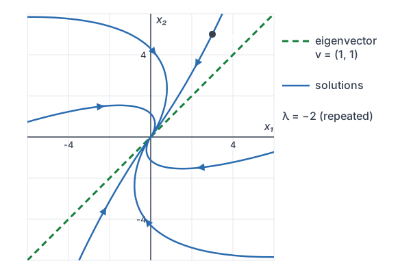
\mathbf{x}(t) = c_1e^{\lambda t}\mathbf{v} + c_2e^{\lambda t}\left(t\mathbf{v} + \mathbf{w}\right)The origin is then an improper node (or degenerate node). It is stable if λ is negative and unstable if λ is positive. As t → ∞, the tv term wins, so solutions become parallel to the eigenvector v.
How to solve x′ = Ax with a repeated eigenvalue
- Solve det(A − λI) = 0 and find the repeated root λ.
- If A = λI, write x = e^(λt)x(0) and stop.
- Find one eigenvector v from (A − λI)v = 0.
- Find a generalized eigenvector w from (A − λI)w = v; any solution works.
- Write x = c₁e^(λt)v + c₂e^(λt)(tv + w), and use c₁v + c₂w = x(0) for an initial-value problem.
Repeated eigenvalues examples
Example 1: A general solution
Find the general solution of x′ = [3 −1; 1 1]x.
\det(A - \lambda I) = (3 - \lambda)(1 - \lambda) + 1
Write the characteristic polynomial: (3 − λ)(1 − λ) − (−1)(1).
(3 - \lambda)(1 - \lambda) + 1 = \lambda^2 - 4\lambda + 4
Multiply out and combine like terms.
\lambda^2 - 4\lambda + 4 = (\lambda - 2)^2
Factor the perfect square trinomial; λ = 2 is repeated.
A - 2I = \begin{bmatrix} 1 & -1 \\ 1 & -1 \end{bmatrix} \Rightarrow v_1 - v_2 = 0Subtract 2 on the diagonal; both rows give the same equation.
\mathbf{v} = \begin{bmatrix} 1 \\ 1 \end{bmatrix}Choose v₁ = 1; there is only one independent eigenvector.
(A - 2I)\mathbf{w} = \mathbf{v}:\ w_1 - w_2 = 1Set up the generalized eigenvector equation; both rows read w₁ − w₂ = 1.
\mathbf{w} = \begin{bmatrix} 1 \\ 0 \end{bmatrix}Choose w₂ = 0, so w₁ = 1.
\mathbf{x} = c_1e^{2t}\begin{bmatrix} 1 \\ 1 \end{bmatrix} + c_2e^{2t}\left(t\begin{bmatrix} 1 \\ 1 \end{bmatrix} + \begin{bmatrix} 1 \\ 0 \end{bmatrix}\right)Write the general solution.
Answer: x(t) = c₁e^(2t)(1, 1) + c₂e^(2t)(t + 1, t). In components, x₁ = e^(2t)(c₁ + c₂ + c₂t) and x₂ = e^(2t)(c₁ + c₂t). Since λ = 2 is positive, the origin is an unstable improper node.
Example 2: An initial-value problem with a stable node
Solve x′ = [−3 1; −1 −1]x with x(0) = (3, 5).
\lambda^2 + 4\lambda + 4 = (\lambda + 2)^2
Trace −4 and determinant 3 + 1 = 4, so det(A − λI) = λ² + 4λ + 4.
A + 2I = \begin{bmatrix} -1 & 1 \\ -1 & 1 \end{bmatrix} \Rightarrow \mathbf{v} = \begin{bmatrix} 1 \\ 1 \end{bmatrix}For λ = −2: −v₁ + v₂ = 0.
-w_1 + w_2 = 1 \Rightarrow \mathbf{w} = \begin{bmatrix} 0 \\ 1 \end{bmatrix}Solve (A + 2I)w = v; choose w₁ = 0.
c_1\begin{bmatrix} 1 \\ 1 \end{bmatrix} + c_2\begin{bmatrix} 0 \\ 1 \end{bmatrix} = \begin{bmatrix} 3 \\ 5 \end{bmatrix}Set t = 0: c₁v + c₂w = x(0).
c_1 = 3,\quad c_1 + c_2 = 5 \Rightarrow c_2 = 2
Read c₁ from the first row, then solve the second.
\mathbf{x} = e^{-2t}\left(3\begin{bmatrix} 1 \\ 1 \end{bmatrix} + 2t\begin{bmatrix} 1 \\ 1 \end{bmatrix} + 2\begin{bmatrix} 0 \\ 1 \end{bmatrix}\right)Substitute c₁ and c₂.
\mathbf{x} = e^{-2t}\begin{bmatrix} 3 + 2t \\ 5 + 2t \end{bmatrix}Add the vectors.
Answer: x₁ = (3 + 2t)e^(−2t) and x₂ = (5 + 2t)e^(−2t). Check: x₁′ = (−4 − 4t)e^(−2t), and −3x₁ + x₂ = (−9 − 6t + 5 + 2t)e^(−2t) = (−4 − 4t)e^(−2t). The solution decays to the origin and comes in parallel to (1, 1).
Example 3: The complete case
Solve x′ = [−1 0; 0 −1]x with x(0) = (2, −3).
\det(A - \lambda I) = (-1 - \lambda)^2 \Rightarrow \lambda = -1
The eigenvalue −1 is repeated.
A + I = \begin{bmatrix} 0 & 0 \\ 0 & 0 \end{bmatrix}Every nonzero vector solves (A + I)v = 0, so A = −I has two independent eigenvectors.
\mathbf{x} = e^{-t}\mathbf{x}(0) = e^{-t}\begin{bmatrix} 2 \\ -3 \end{bmatrix}Each equation is xᵢ′ = −xᵢ on its own.
Answer: x = e^(−t)(2, −3). No t-term appears, and the solution moves straight toward the origin along the line through (2, −3). The origin is a stable star. For a 2 × 2 matrix, this complete case happens only when A is a multiple of I.
Example 4: Two tanks in a row (word problem)
Two 100 L tanks are connected in a row. Pure water flows into tank 1 at 5 L/min, the mixture flows from tank 1 into tank 2 at 5 L/min, and it leaves tank 2 at 5 L/min. Tank 1 starts with 10 kg of salt and tank 2 with none. Find x₁(t) and x₂(t), and find when tank 2 holds the most salt.
x_1' = -0.05x_1,\quad x_2' = 0.05x_1 - 0.05x_2
Salt leaves each tank at (amount/100)(5) kg/min, as in mixing problems.
\lambda = -0.05 \text{ (repeated)}A = [−0.05 0; 0.05 −0.05] is triangular, so read the diagonal.
A + 0.05I = \begin{bmatrix} 0 & 0 \\ 0.05 & 0 \end{bmatrix} \Rightarrow \mathbf{v} = \begin{bmatrix} 0 \\ 1 \end{bmatrix}The equation 0.05v₁ = 0 forces v₁ = 0.
0.05w_1 = 1 \Rightarrow \mathbf{w} = \begin{bmatrix} 20 \\ 0 \end{bmatrix}Solve (A + 0.05I)w = v; choose w₂ = 0.
c_1\begin{bmatrix} 0 \\ 1 \end{bmatrix} + c_2\begin{bmatrix} 20 \\ 0 \end{bmatrix} = \begin{bmatrix} 10 \\ 0 \end{bmatrix} \Rightarrow c_1 = 0,\ c_2 = 0.5Set t = 0 and match x(0) = (10, 0).
\mathbf{x} = 0.5e^{-0.05t}\left(t\begin{bmatrix} 0 \\ 1 \end{bmatrix} + \begin{bmatrix} 20 \\ 0 \end{bmatrix}\right) = e^{-0.05t}\begin{bmatrix} 10 \\ 0.5t \end{bmatrix}Substitute and multiply by 0.5.
x_2' = 0.5e^{-0.05t}(1 - 0.05t)Differentiate x₂ = 0.5te^(−0.05t) with the product rule and factor.
1 - 0.05t = 0 \Rightarrow t = 20
Set x₂′ = 0; e^(−0.05t) is never 0.
x_2(20) = 0.5(20)e^{-1} = 10e^{-1} \approx 3.68Substitute t = 20.
Answer: x₁ = 10e^(−0.05t) and x₂ = 0.5te^(−0.05t) kilograms. Tank 2 holds the most salt, about 3.68 kg, at t = 20 minutes. Equal outflow rates give equal diagonal entries, which is why the eigenvalue repeats and t appears in the answer.
Example 5: Critical damping as a system
Write y″ + 6y′ + 9y = 0 with y(0) = 1 and y′(0) = 0 as a system, solve it, and compare with the scalar method.
\mathbf{x}' = \begin{bmatrix} 0 & 1 \\ -9 & -6 \end{bmatrix}\mathbf{x}Let x₁ = y and x₂ = y′, as in systems of differential equations.
\lambda^2 + 6\lambda + 9 = (\lambda + 3)^2
det(A − λI) = −λ(−6 − λ) + 9; λ = −3 is repeated.
A + 3I = \begin{bmatrix} 3 & 1 \\ -9 & -3 \end{bmatrix} \Rightarrow \mathbf{v} = \begin{bmatrix} 1 \\ -3 \end{bmatrix}The first row gives 3v₁ + v₂ = 0.
3w_1 + w_2 = 1 \Rightarrow \mathbf{w} = \begin{bmatrix} 0 \\ 1 \end{bmatrix}Solve (A + 3I)w = v; choose w₁ = 0.
c_1\begin{bmatrix} 1 \\ -3 \end{bmatrix} + c_2\begin{bmatrix} 0 \\ 1 \end{bmatrix} = \begin{bmatrix} 1 \\ 0 \end{bmatrix} \Rightarrow c_1 = 1,\ c_2 = 3The first row gives c₁ = 1; the second gives −3 + c₂ = 0.
\mathbf{x} = e^{-3t}\left(\begin{bmatrix} 1 \\ -3 \end{bmatrix} + 3t\begin{bmatrix} 1 \\ -3 \end{bmatrix} + 3\begin{bmatrix} 0 \\ 1 \end{bmatrix}\right)Substitute c₁ and c₂.
\mathbf{x} = e^{-3t}\begin{bmatrix} 1 + 3t \\ -9t \end{bmatrix}Add the vectors.
Answer: y = x₁ = (1 + 3t)e^(−3t), and the velocity is y′ = x₂ = −9te^(−3t). This is the same answer the scalar method gives in repeated roots of the characteristic equation: the te^(rt) term there is the tv term here.
Common mistakes
| Mistake | Example of the error | Fix |
|---|---|---|
| Using te^(λt)v as the second solution | x = c₁e^(2t)(1, 1) + c₂te^(2t)(1, 1) | Add e^(λt)w: the second solution is e^(λt)(tv + w). |
| Solving (A − λI)w = 0 for w | Getting w = (1, 1) again, the same as v | Solve (A − λI)w = v, with v on the right side. |
| Putting t on the wrong vector | e^(λt)(v + tw) | The t goes with the eigenvector: e^(λt)(tv + w). |
| Assuming every repeated eigenvalue is defective | Adding a t-term for A = −I | If A − λI is the zero matrix, every vector is an eigenvector and x = e^(λt)x(0). |
| Using t = 0 incorrectly in the initial values | c₁v + c₂(v + w) = x(0) | At t = 0, tv is the zero vector: c₁v + c₂w = x(0). |
| Thinking w must be unique | Calling w = (2, 1) wrong when the answer key has (1, 0) | Any w with (A − λI)w = v works; only c₁ changes. |
Related ideas
Where repeated eigenvalues sit among the cases
For a 2 × 2 matrix, the eigenvalues repeat exactly when (tr A)² − 4 det A = 0. This is the border between two real eigenvalues, from solving linear systems with eigenvalues, and a complex pair, from complex eigenvalues. An improper node looks like a spiral that does not quite turn. Phase Portraits compares all of these pictures.
Larger systems
In an n × n system, an eigenvalue can repeat more than twice. Then you may need a chain of generalized eigenvectors, (A − λI)w₁ = v and (A − λI)w₂ = w₁, which give solutions with t²/2 terms. These chains are the idea behind the Jordan form in linear algebra.
Practice problems
- Find the eigenvalues of A = [5 −4; 1 1].
- For A = [5 −4; 1 1], find an eigenvector v and a generalized eigenvector w.
- Write the general solution of x′ = [5 −4; 1 1]x.
- Solve x′ = [−2 0; 0 −2]x with x(0) = (4, 1).
- Solve x′ = [1 1; 0 1]x with x(0) = (2, 3).
- For A = [3 −1; 1 1], λ = 2 and v = (1, 1), show that te^(2t)v alone is not a solution of x′ = Ax.
- Write y″ − 4y′ + 4y = 0 as a system, find v and w, and give y(t).
- Classify the origin for x′ = [3 −1; 1 1]x and for x′ = [−1 0; 0 −1]x.
- Two 200 L tanks are in a row with water flowing at 10 L/min, pure water entering tank 1. Tank 1 starts with 20 kg of salt and tank 2 with none. Find x₂(t) and its maximum.
- In Example 1, show that w = (2, 1) is also a generalized eigenvector, and explain why it gives the same solutions.
Show answers
1.
\lambda^2 - 6\lambda + 9 = 0
Trace 6 and determinant 5 + 4 = 9.
(\lambda - 3)^2 = 0 \Rightarrow \lambda = 3
Factor the perfect square.
Answer: λ = 3, repeated
2.
A - 3I = \begin{bmatrix} 2 & -4 \\ 1 & -2 \end{bmatrix} \Rightarrow \mathbf{v} = \begin{bmatrix} 2 \\ 1 \end{bmatrix}The second row gives v₁ − 2v₂ = 0.
w_1 - 2w_2 = 1 \Rightarrow \mathbf{w} = \begin{bmatrix} 1 \\ 0 \end{bmatrix}Solve (A − 3I)w = v using the second row; row 1 is twice row 2.
Answer: v = (2, 1) and w = (1, 0)
3.
\mathbf{x} = c_1e^{3t}\begin{bmatrix} 2 \\ 1 \end{bmatrix} + c_2e^{3t}\left(t\begin{bmatrix} 2 \\ 1 \end{bmatrix} + \begin{bmatrix} 1 \\ 0 \end{bmatrix}\right)Use v and w from Problem 2.
Answer: x = c₁e^(3t)(2, 1) + c₂e^(3t)(2t + 1, t)
4.
A = -2I \Rightarrow \mathbf{x} = e^{-2t}\mathbf{x}(0)The complete case: every vector is an eigenvector.
Answer: x = e^(−2t)(4, 1)
5.
A - I = \begin{bmatrix} 0 & 1 \\ 0 & 0 \end{bmatrix} \Rightarrow \mathbf{v} = \begin{bmatrix} 1 \\ 0 \end{bmatrix},\ \mathbf{w} = \begin{bmatrix} 0 \\ 1 \end{bmatrix}λ = 1 is repeated; v₂ = 0 for v, and w₂ = 1 for w.
c_1 = 2,\quad c_2 = 3
Match c₁(1, 0) + c₂(0, 1) = (2, 3).
\mathbf{x} = e^{t}\left(2\begin{bmatrix} 1 \\ 0 \end{bmatrix} + 3t\begin{bmatrix} 1 \\ 0 \end{bmatrix} + 3\begin{bmatrix} 0 \\ 1 \end{bmatrix}\right)Substitute the constants.
Answer: x = e^t(2 + 3t, 3)
6.
\left(te^{2t}\mathbf{v}\right)' = (1 + 2t)e^{2t}\mathbf{v}Product rule.
A\left(te^{2t}\mathbf{v}\right) = te^{2t}A\mathbf{v} = 2te^{2t}\mathbf{v}Use Av = 2v.
Answer: the two sides differ by e^(2t)v = e^(2t)(1, 1), so it is not a solution
7.
\mathbf{x}' = \begin{bmatrix} 0 & 1 \\ -4 & 4 \end{bmatrix}\mathbf{x},\quad (\lambda - 2)^2 = 0Let x₁ = y, x₂ = y′; det(A − λI) = λ² − 4λ + 4.
\mathbf{v} = \begin{bmatrix} 1 \\ 2 \end{bmatrix},\quad \mathbf{w} = \begin{bmatrix} 0 \\ 1 \end{bmatrix}Row 1 of A − 2I: −2v₁ + v₂ = 0, and −2w₁ + w₂ = 1.
y = x_1 = c_1e^{2t} + c_2te^{2t}First entries of c₁e^(2t)v + c₂e^(2t)(tv + w).
Answer: y = (c₁ + c₂t)e^(2t)
8.
\lambda = 2 \gt 0 \text{ with one eigenvector}First matrix, from Example 1.
\lambda = -1 \lt 0,\ A = -I
Second matrix.
Answer: unstable improper node; stable star (proper node)
9.
x_1' = -0.05x_1,\quad x_2' = 0.05x_1 - 0.05x_2
10/200 = 0.05; same matrix as Example 4.
c_1 = 0,\quad 20c_2 = 20 \Rightarrow c_2 = 1
With v = (0, 1) and w = (20, 0), match x(0) = (20, 0).
\mathbf{x} = e^{-0.05t}\begin{bmatrix} 20 \\ t \end{bmatrix}e^(−0.05t)(t(0, 1) + (20, 0)).
x_2' = e^{-0.05t}(1 - 0.05t) = 0 \Rightarrow t = 20Product rule; set the derivative to 0.
Answer: x₂ = te^(−0.05t) kg, with a maximum of 20e^(−1) ≈ 7.36 kg at t = 20 min
10.
(A - 2I)\begin{bmatrix} 2 \\ 1 \end{bmatrix} = \begin{bmatrix} 2 - 1 \\ 2 - 1 \end{bmatrix} = \begin{bmatrix} 1 \\ 1 \end{bmatrix}Multiply [1 −1; 1 −1] by (2, 1).
(2, 1) = (1, 0) + (1, 1)
The new w is the old w plus v.
Answer: (2, 1) works; c₂e^(2t)(tv + w + v) = c₂e^(2t)(tv + w) + c₂e^(2t)v, and the extra c₂e^(2t)v joins the c₁ term
Repeated eigenvalues FAQ
What is a generalized eigenvector?
It is a vector w with (A − λI)w = v, where v is an eigenvector for λ. It is not an eigenvector itself, but A − λI sends it to one. It supplies the missing second solution when an eigenvalue repeats.
Why is the second solution te^(λt)v + e^(λt)w?
Substituting te^(λt)v into x′ = Ax leaves an extra e^(λt)v. Adding e^(λt)w cancels it exactly when (A − λI)w = v.
What if a repeated eigenvalue has two eigenvectors?
Then there is no t-term: x = c₁e^(λt)v₁ + c₂e^(λt)v₂. For a 2 × 2 matrix this happens only when A = λI, and every solution is e^(λt)x(0).
What does the phase portrait look like for a repeated eigenvalue?
With one eigenvector, the origin is an improper node: solutions approach (λ < 0) or leave (λ > 0) along curves that become parallel to the eigenvector. With A = λI, it is a star, with straight-line solutions in every direction.
Summary
- A repeated eigenvalue λ usually has only one eigenvector v.
- Find a generalized eigenvector w from (A − λI)w = v.
- The general solution is x = c₁e^(λt)v + c₂e^(λt)(tv + w); at t = 0, c₁v + c₂w = x(0).
- If A = λI, the solution is simply x = e^(λt)x(0).
- The origin is an improper node (one eigenvector) or a star (A = λI), stable when λ is negative.
Previous lesson: Complex Eigenvalues
Next lesson: Phase Portraits
Back to the Differential Equations Index