
Reduction of Order
Reduction of order finds a second solution of a second-order linear homogeneous equation when you already know one solution y₁. Substitute y₂ = v(x)y₁(x). The terms with v itself cancel, leaving a first-order equation for w = v′. Solve for w, integrate to get v, and then y₂ = vy₁.
Before this lesson: Second-Order Homogeneous Linear Equations, The Wronskian and Separable Differential Equations
The idea: multiply the known solution by a function
If y₁ solves the equation, so does Cy₁ for any constant C. Those are not new, though. To get a different solution, let the constant become a function: try y = v(x)y₁(x).
When you substitute, every term that still contains v (not v′ or v″) collects into v times the original equation applied to y₁. That is 0, because y₁ is a solution. Only v′ and v″ remain, so setting w = v′ lowers the order from 2 to 1. That is where the name comes from.
Any nonconstant v works, so you can drop constants of integration along the way. The result y₂ = vy₁ is not a constant multiple of y₁, so {y₁, y₂} is a fundamental set.
Reduction of order formula
For y″ + p(x)y′ + q(x)y = 0 with a known solution y₁, substituting y = vy₁ gives
y_1v'' + \left(2y_1' + p\,y_1\right)v' = 0 \quad\Longrightarrow\quad v' = \dfrac{e^{-\int p(x)\,dx}}{y_1^2}y_2 = y_1\displaystyle\int \dfrac{e^{-\int p(x)\,dx}}{y_1^2}\,dxThe equation must be in standard form, with the coefficient of y″ equal to 1, before you read off p(x).
How to use reduction of order
- Write the equation in standard form y″ + p(x)y′ + q(x)y = 0 and identify p.
- Compute e^(−∫p dx), dropping the constant.
- Divide by y₁² to get v′, then integrate to get v (again dropping the constant).
- Multiply: y₂ = vy₁. The general solution is y = C₁y₁ + C₂y₂.
You can also substitute y = vy₁ directly, as in Examples 1 and 2. That is longer but shows why the method works.
Reduction of order examples
Example 1: A repeated root, by direct substitution
The equation y″ − 4y′ + 4y = 0 has the solution y₁ = e^(2x). Find a second solution.
y = ve^{2x}Let the constant multiplier become a function v(x).
y' = v'e^{2x} + 2ve^{2x}Differentiate with the product rule.
y'' = v''e^{2x} + 4v'e^{2x} + 4ve^{2x}Differentiate again and combine the two v′e^(2x) terms.
v''e^{2x} + 4v'e^{2x} + 4ve^{2x} - 4v'e^{2x} - 8ve^{2x} + 4ve^{2x} = 0Substitute into y″ − 4y′ + 4y = 0 and distribute.
v''e^{2x} = 0Combine like terms: the v′ terms and the v terms both cancel.
v'' = 0
Divide both sides by e^(2x), which is never 0.
v = x
Integrate twice, keeping the simplest nonconstant choice.
y_2 = xe^{2x}Multiply v by y₁.
Answer: y₂ = xe^(2x), and the general solution is y = (C₁ + C₂x)e^(2x). The characteristic equation r² − 4r + 4 = 0 has the repeated root 2, which is why the usual method gives only one exponential.
Example 2: Variable coefficients, by direct substitution
For positive x, y₁ = x² solves x²y″ − 3xy′ + 4y = 0. Find a second solution.
y = vx^2,\quad y' = v'x^2 + 2xv
Substitute y = vx² and differentiate with the product rule.
y'' = v''x^2 + 4xv' + 2v
Differentiate again and combine like terms.
x^4v'' + 4x^3v' + 2x^2v - 3x^3v' - 6x^2v + 4x^2v = 0
Substitute into the equation and distribute.
x^4v'' + x^3v' = 0
Combine like terms: the v terms cancel.
xw' + w = 0
Let w = v′ and divide both sides by x³.
\dfrac{dw}{w} = -\dfrac{dx}{x}Separate the variables.
\ln w = -\ln x \Rightarrow w = \dfrac{1}{x}Integrate both sides and exponentiate, dropping the constant (see properties of logarithms).
v = \ln x
Integrate w = 1/x (see integrals that give natural logarithms).
y_2 = x^2\ln x
Multiply v by y₁.
Answer: y₂ = x² ln x, so y = C₁x² + C₂x² ln x for positive x.
Example 3: Using the formula
For positive x, y₁ = x solves x²y″ + xy′ − y = 0. Use the formula to find a second solution.
y'' + \dfrac{1}{x}y' - \dfrac{1}{x^2}y = 0Divide by x² to get standard form, so p(x) = 1/x.
e^{-\int p\,dx} = e^{-\ln x} = \dfrac{1}{x}Integrate p and use e^(−ln x) = 1/x.
v' = \dfrac{1/x}{x^2} = x^{-3}Divide by y₁² = x².
v = \dfrac{x^{-2}}{-2} = -\dfrac{1}{2x^2}Integrate with the power rule.
y_2 = x\left(-\dfrac{1}{2x^2}\right) = -\dfrac{1}{2x}Multiply v by y₁.
y_2 = \dfrac{1}{x}Drop the constant factor −1/2; any multiple of a solution is a solution.
Answer: y₂ = 1/x. Check: y′ = −1/x² and y″ = 2/x³, so x²(2/x³) + x(−1/x²) − 1/x = 2/x − 1/x − 1/x = 0.
Example 4: A formula integral that needs integration by parts
The function y₁ = e^x solves xy″ − (x + 1)y′ + y = 0 for positive x. Find a second solution.
y'' - \left(1 + \dfrac{1}{x}\right)y' + \dfrac{1}{x}y = 0Divide by x, so p(x) = −(1 + 1/x).
e^{-\int p\,dx} = e^{x + \ln x} = xe^{x}Integrate 1 + 1/x to get x + ln x, then use e^(ln x) = x.
v' = \dfrac{xe^{x}}{e^{2x}} = xe^{-x}Divide by y₁² = e^(2x).
v = -xe^{-x} - e^{-x}Integrate by parts with u = x, dv = e^(−x) dx (see integration by parts).
y_2 = e^{x}\left(-xe^{-x} - e^{-x}\right) = -x - 1Multiply v by y₁.
y_2 = x + 1
Drop the factor −1.
Answer: y₂ = x + 1. Check: y′ = 1 and y″ = 0, so x(0) − (x + 1)(1) + (x + 1) = 0.
Example 5: A critically damped spring (word problem)
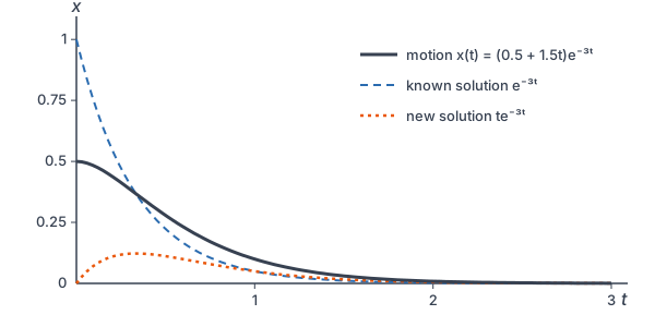
A spring’s position x (in meters) satisfies x″ + 6x′ + 9x = 0, with t in seconds, and one solution is x₁ = e^(−3t). Find a second solution, then the motion with x(0) = 0.5 and x′(0) = 0.
e^{-\int 6\,dt} = e^{-6t}Standard form already holds, with p = 6.
v' = \dfrac{e^{-6t}}{\left(e^{-3t}\right)^2} = 1Divide by x₁² = e^(−6t).
v = t,\quad x_2 = te^{-3t}Integrate and multiply by x₁.
x = (C_1 + C_2t)e^{-3t}Write the general solution.
x' = C_2e^{-3t} - 3(C_1 + C_2t)e^{-3t}Differentiate with the product rule.
C_1 = 0.5
Substitute t = 0 into x.
C_2 - 3(0.5) = 0 \Rightarrow C_2 = 1.5
Substitute t = 0 into x′ and solve.
x = (0.5 + 1.5t)e^{-3t}Write the motion.
x(1) = 2e^{-3} \approx 0.0996For example, substitute t = 1.
Answer: x₂ = te^(−3t) and x(t) = (0.5 + 1.5t)e^(−3t). After 1 second the spring is about 0.1 m from rest position, and it returns without ever overshooting.
Common mistakes
| Mistake | Example of the error | Fix |
|---|---|---|
| Reading p before dividing by the leading coefficient | Using p = −3x for x²y″ − 3xy′ + 4y = 0 | Divide by x² first: p = −3/x. |
| Forgetting the product rule | Writing (vy₁)′ = v′y₁′ | (vy₁)′ = v′y₁ + vy₁′. |
| Stopping at v | Giving v = ln x as the second solution | The second solution is y₂ = vy₁ = x² ln x. |
| Choosing a constant v | Taking v = 5 | A constant v only gives 5y₁. Choose a nonconstant antiderivative. |
| Forgetting the minus sign in e^(−∫p dx) | Using e^(∫p dx) | The formula uses e^(−∫p dx), the same factor as Abel’s formula for the Wronskian. |
| Dividing by y₁ instead of y₁² | v′ = e^(−∫p dx)/y₁ | Divide by y₁ squared. |
Related ideas
Why the formula works
The Wronskian of y₁ and y₂ = vy₁ is W = y₁(v′y₁ + vy₁′) − vy₁y₁′ = v′y₁². By Abel’s formula from the Wronskian lesson, W = e^(−∫p dx) up to a constant. Setting them equal gives v′ = e^(−∫p dx)/y₁².
Repeated roots
Examples 1 and 5 show the pattern for a repeated root r of the characteristic equation: the second solution is xe^(rx). Repeated Roots of the Characteristic Equation uses this as a rule.
Equations with nonconstant coefficients
For constant coefficients, the characteristic equation is faster. Reduction of order earns its keep when the coefficients depend on x, as in Examples 2 to 4, and for Cauchy-Euler Equations.
Practice problems
- Given y₁ = e^(−x), find a second solution of y″ + 2y′ + y = 0.
- Given y₁ = e^(3x), find a second solution of y″ − 6y′ + 9y = 0.
- For positive x, y₁ = x solves x²y″ − xy′ + y = 0. Find a second solution.
- For positive x, y₁ = x³ solves x²y″ − 5xy′ + 9y = 0. Find a second solution.
- For positive x, y₁ = x solves x²y″ + 2xy′ − 2y = 0. Find a second solution.
- Given y₁ = e^x, use reduction of order to find a second solution of y″ − y = 0.
- On the interval from 0 to π, y₁ = sin x solves y″ + y = 0. Use reduction of order to find a second solution.
- Given y₁ = e^(x/2), find the general solution of 4y″ − 4y′ + y = 0.
- Show that substituting y = vy₁ into y″ + py′ + qy = 0 gives y₁v″ + (2y₁′ + py₁)v′ = 0.
- A spring satisfies x″ + 4x′ + 4x = 0 with x₁ = e^(−2t), x(0) = 1 and x′(0) = 3. Find x(t) and the time of the largest displacement.
Show answers
1.
v' = \dfrac{e^{-2x}}{e^{-2x}} = 1p = 2, so e^(−∫p dx) = e^(−2x); divide by y₁² = e^(−2x).
v = x
Integrate.
Answer: y₂ = xe^(−x)
2.
v' = \dfrac{e^{6x}}{e^{6x}} = 1p = −6, so e^(−∫p dx) = e^(6x); divide by y₁² = e^(6x).
v = x
Integrate.
Answer: y₂ = xe^(3x)
3.
p = -\dfrac{1}{x},\quad e^{-\int p\,dx} = e^{\ln x} = xDivide by x² for standard form, then integrate p.
v' = \dfrac{x}{x^2} = \dfrac{1}{x}Divide by y₁² = x².
v = \ln x
Integrate.
Answer: y₂ = x ln x
4.
p = -\dfrac{5}{x},\quad e^{-\int p\,dx} = e^{5\ln x} = x^5Divide by x², integrate p, and use 5 ln x = ln x⁵.
v' = \dfrac{x^5}{x^6} = \dfrac{1}{x}Divide by y₁² = x⁶.
v = \ln x
Integrate.
Answer: y₂ = x³ ln x
5.
p = \dfrac{2}{x},\quad e^{-\int p\,dx} = e^{-2\ln x} = x^{-2}Divide by x² and integrate p.
v' = \dfrac{x^{-2}}{x^2} = x^{-4}Divide by y₁² = x².
v = -\dfrac{x^{-3}}{3}Integrate with the power rule.
y_2 = x\left(-\dfrac{1}{3x^3}\right) = -\dfrac{1}{3x^2}Multiply by y₁.
Answer: y₂ = 1/x² (dropping the factor −1/3)
6.
v' = \dfrac{1}{e^{2x}} = e^{-2x}p = 0, so e^(−∫p dx) = 1; divide by y₁² = e^(2x).
v = -\tfrac{1}{2}e^{-2x}Integrate.
y_2 = e^{x}\left(-\tfrac{1}{2}e^{-2x}\right) = -\tfrac{1}{2}e^{-x}Multiply by y₁.
Answer: y₂ = e^(−x) (dropping the factor −1/2)
7.
v' = \dfrac{1}{\sin^2 x} = \csc^2 xp = 0; divide 1 by y₁² = sin² x.
v = -\cot x
Integrate: the derivative of cot x is −csc² x.
y_2 = \sin x(-\cot x) = -\cos x
Multiply by y₁ and use cot x = cos x/sin x.
Answer: y₂ = cos x (dropping the factor −1)
8.
y'' - y' + \tfrac{1}{4}y = 0Divide by 4, so p = −1.
v' = \dfrac{e^{x}}{e^{x}} = 1e^(−∫p dx) = e^x, and y₁² = e^x.
v = x
Integrate.
Answer: y = (C₁ + C₂x)e^(x/2)
9.
y' = v'y_1 + vy_1',\quad y'' = v''y_1 + 2v'y_1' + vy_1''
Differentiate y = vy₁ twice with the product rule.
y_1v'' + (2y_1' + py_1)v' + v(y_1'' + py_1' + qy_1) = 0
Substitute into y″ + py′ + qy = 0 and group by v″, v′ and v.
y_1v'' + (2y_1' + py_1)v' = 0
The last group is 0 because y₁ is a solution.
Answer: the v terms drop out, leaving y₁v″ + (2y₁′ + py₁)v′ = 0
10.
v' = \dfrac{e^{-4t}}{e^{-4t}} = 1 \Rightarrow x_2 = te^{-2t}p = 4; divide e^(−4t) by x₁² = e^(−4t) and integrate.
x = (C_1 + C_2t)e^{-2t},\quad C_1 = 1Write the general solution and substitute t = 0.
x' = C_2e^{-2t} - 2(C_1 + C_2t)e^{-2t}Differentiate with the product rule.
C_2 - 2 = 3 \Rightarrow C_2 = 5
Substitute t = 0 and C₁ = 1 into x′.
x' = (5 - 2 - 10t)e^{-2t} = (3 - 10t)e^{-2t}Substitute the constants into x′ and simplify.
t = 0.3,\quad x(0.3) = 2.5e^{-0.6} \approx 1.372Set x′ = 0, then evaluate x at t = 0.3.
Answer: x(t) = (1 + 5t)e^(−2t); the largest displacement is about 1.372 at t = 0.3 s
Reduction of order FAQ
What is reduction of order?
It is a method for finding a second solution of a second-order linear homogeneous differential equation when one solution y₁ is known. You set y₂ = v(x)y₁ and solve a first-order equation for v′.
What is the reduction of order formula?
For y″ + p(x)y′ + q(x)y = 0, the second solution is y₂ = y₁∫(e^(−∫p dx)/y₁²) dx. The equation must be in standard form first.
Why is it called reduction of order?
After substituting y = vy₁, the terms with v cancel and only v′ and v″ remain. Letting w = v′ turns the second-order equation into a first-order one.
When do you use reduction of order?
Use it when you know one solution but not a second, especially for equations with variable coefficients and for repeated roots of a characteristic equation.
Summary
- Reduction of order finds a second solution y₂ = vy₁ from a known solution y₁.
- Substituting y = vy₁ cancels the v terms and leaves a first-order equation for w = v′.
- Shortcut: v′ = e^(−∫p dx)/y₁², with the equation in standard form.
- Drop constants of integration and constant factors; any nonconstant v works.
- The general solution is y = C₁y₁ + C₂y₂.
Previous lesson: The Wronskian
Next lesson: Complex Roots of the Characteristic Equation
Back to the Differential Equations Index