
Boundary Value Problems
A boundary value problem gives conditions at two different points, such as y(0) = 0 and y(L) = 0, instead of at one starting point. Unlike an initial value problem, it can have one solution, no solution or infinitely many. When the equation has a parameter λ, the values of λ that allow nonzero solutions are its eigenvalues.
Before this lesson: Second-Order Homogeneous Linear Equations, Complex Roots of the Characteristic Equation and Existence and Uniqueness Theorem
Initial value problems vs. boundary value problems
An initial value problem fixes y and y′ at one point, like launching a ball from a known spot at a known velocity. The existence and uniqueness theorem then promises exactly one solution.
A boundary value problem fixes y (or y′) at two ends of an interval, like a string tied down at both ends. Now there is no guarantee. You still find the general solution first, but the two conditions can agree, clash, or leave a constant undecided.
How to solve boundary value problems
- Find the general solution, such as y = c₁ cos kx + c₂ sin kx.
- Substitute each boundary condition to get two equations in c₁ and c₂.
- Solve that system. A single solution means the problem has exactly one solution.
- If the conditions contradict each other (such as 0 = 2), there is no solution. If one equation reads 0 = 0, a constant can take any value and there are infinitely many solutions.
Eigenvalue problems
Many boundary value problems contain a parameter λ, as in y″ + λy = 0 with y(0) = 0 and y(L) = 0. The zero function y = 0 always solves it. The values of λ that also allow a nonzero solution are the eigenvalues, and those nonzero solutions are the eigenfunctions.
This matches eigenvalues and eigenvectors in linear algebra: the equation −y″ = λy says the operator −d²/dx² turns y into a multiple of itself. To find the eigenvalues, test three cases: λ < 0, λ = 0 and λ > 0.
y'' + \lambda y = 0,\quad y(0) = 0,\quad y(L) = 0 \quad\Longrightarrow\quad \lambda_n = \left(\frac{n\pi}{L}\right)^2,\quad y_n = \sin\frac{n\pi x}{L},\quad n = 1, 2, 3, \ldotsThe table lists the three eigenvalue problems for y″ + λy = 0 on 0 ≤ x ≤ L that come up most often. Each eigenfunction can be multiplied by any nonzero constant.
| Boundary conditions | Eigenvalues | Eigenfunctions |
|---|---|---|
| y(0) = 0,\ y(L) = 0 | \lambda_n = (n\pi/L)^2,\ n = 1, 2, 3, \ldots | \sin(n\pi x/L) |
| y'(0) = 0,\ y'(L) = 0 | \lambda_n = (n\pi/L)^2,\ n = 0, 1, 2, \ldots | \cos(n\pi x/L); y_0 = 1 |
| y(0) = 0,\ y'(L) = 0 | \lambda_n = \left(\frac{(2n-1)\pi}{2L}\right)^2,\ n = 1, 2, 3, \ldots | \sin\left(\frac{(2n-1)\pi x}{2L}\right) |
Boundary value problem examples
Example 1: A boundary value problem with one solution
Solve y″ + 4y = 0 with y(0) = 1 and y(π/4) = 3.
r^2 + 4 = 0 \Rightarrow r = \pm 2i
Write the characteristic equation and solve it.
y = c_1\cos 2x + c_2\sin 2x
Use the complex roots form with α = 0 and β = 2.
y(0) = c_1\cos 0 + c_2\sin 0 = c_1
Substitute x = 0.
c_1 = 1
Use y(0) = 1.
y\left(\frac{\pi}{4}\right) = c_1\cos\frac{\pi}{2} + c_2\sin\frac{\pi}{2} = c_2Substitute x = π/4; cos(π/2) = 0 and sin(π/2) = 1 (trig values of special angles).
c_2 = 3
Use y(π/4) = 3.
Answer: y = cos 2x + 3 sin 2x. The two conditions fixed both constants, so this is the only solution.
Example 2: No solution or infinitely many solutions
Keep y″ + 4y = 0 and y(0) = 1, but move the second condition to x = π. Solve the problem with (a) y(π) = 2 and (b) y(π) = 1.
y = c_1\cos 2x + c_2\sin 2x,\quad c_1 = 1
Same general solution, and y(0) = 1 still gives c₁ = 1.
y(\pi) = c_1\cos 2\pi + c_2\sin 2\pi = c_1
Substitute x = π; cos 2π = 1 and sin 2π = 0.
\text{(a)}\quad c_1 = 2Use y(π) = 2.
1 = 2
Both conditions fix c₁, and they disagree.
\text{(b)}\quad c_1 = 1Use y(π) = 1.
1 = 1
This agrees with c₁ = 1, and c₂ never appears.
Answer: (a) has no solution. (b) has infinitely many solutions, y = cos 2x + c₂ sin 2x for any c₂. The reason is that sin 2x is 0 at both x = 0 and x = π, so any multiple of it can be added without changing either boundary value.
Example 3: Eigenvalues with y(0) = 0 and y(2) = 0
Find the eigenvalues and eigenfunctions of y″ + λy = 0 with y(0) = 0 and y(2) = 0.
\lambda = -\mu^2 \lt 0:\quad y = c_1\cosh\mu x + c_2\sinh\mu x
Case 1: the roots are r = ±μ; write the solution with hyperbolic functions.
y(0) = c_1 = 0
cosh 0 = 1 and sinh 0 = 0.
y(2) = c_2\sinh 2\mu = 0 \Rightarrow c_2 = 0
sinh 2μ ≠ 0 when μ > 0, so only y = 0 works.
\lambda = 0:\quad y = c_1 + c_2x
Case 2: y″ = 0, so y is linear.
y(0) = c_1 = 0,\quad y(2) = 2c_2 = 0
Both constants are 0, so λ = 0 is not an eigenvalue.
\lambda = \mu^2 \gt 0:\quad y = c_1\cos\mu x + c_2\sin\mu x
Case 3: the roots are r = ±μi.
y(0) = c_1 = 0
Substitute x = 0.
y(2) = c_2\sin 2\mu = 0
Substitute x = 2; take c₂ ≠ 0 to get a nonzero solution.
2\mu = n\pi \Rightarrow \mu = \frac{n\pi}{2},\quad n = 1, 2, 3, \ldotsSine is 0 at whole multiples of π (solving trig equations); μ > 0, so n ≥ 1.
\lambda_n = \mu^2 = \frac{n^2\pi^2}{4}Square μ.
Answer: λₙ = n²π²/4 with eigenfunctions yₙ = sin(nπx/2), for n = 1, 2, 3, …. The first three eigenvalues are π²/4 ≈ 2.467, π² ≈ 9.870 and 9π²/4 ≈ 22.207. Each eigenfunction fits n half-waves between x = 0 and x = 2, as the graph shows.
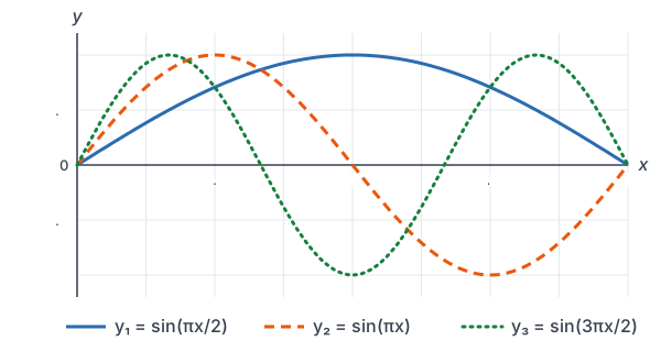
Example 4: Eigenvalues with y′(0) = 0 and y′(π) = 0
Find the eigenvalues and eigenfunctions of y″ + λy = 0 with y′(0) = 0 and y′(π) = 0.
\lambda = -\mu^2:\quad y' = c_1\mu\sinh\mu x + c_2\mu\cosh\mu x
Case 1: differentiate y = c₁ cosh μx + c₂ sinh μx.
y'(0) = c_2\mu = 0 \Rightarrow c_2 = 0
μ > 0.
y'(\pi) = c_1\mu\sinh\mu\pi = 0 \Rightarrow c_1 = 0
sinh μπ ≠ 0, so there is no negative eigenvalue.
\lambda = 0:\quad y = c_1 + c_2x,\quad y' = c_2
Case 2: y is linear.
y'(0) = c_2 = 0
Both conditions just say c₂ = 0, and c₁ can be any number.
\lambda_0 = 0,\quad y_0 = 1
A nonzero constant works, so 0 is an eigenvalue.
\lambda = \mu^2:\quad y' = -c_1\mu\sin\mu x + c_2\mu\cos\mu x
Case 3: differentiate y = c₁ cos μx + c₂ sin μx.
y'(0) = c_2\mu = 0 \Rightarrow c_2 = 0
μ > 0.
y'(\pi) = -c_1\mu\sin\mu\pi = 0
Take c₁ ≠ 0.
\mu\pi = n\pi \Rightarrow \mu = n,\quad \lambda_n = n^2
Sine is 0 at whole multiples of π; square μ.
Answer: λₙ = n² with eigenfunctions yₙ = cos nx, for n = 0, 1, 2, …. With conditions on y′ (called Neumann conditions), λ = 0 is an eigenvalue and its eigenfunction is the constant 1.
Example 5: Buckling of a column (word problem)
A thin vertical rod 1.5 meters long is pinned at both ends and pressed from above by a load P (in newtons). Its sideways bend y(x) satisfies EIy″ + Py = 0 with y(0) = 0 and y(1.5) = 0, where the stiffness is EI = 450 N·m². The rod stays straight unless the problem has a nonzero solution. Find the smallest load that makes the rod buckle.
y'' + \frac{P}{EI}y = 0Divide by EI; this is y″ + λy = 0 with λ = P/EI.
\lambda_n = \left(\frac{n\pi}{1.5}\right)^2Use the eigenvalues for y(0) = 0 and y(L) = 0 with L = 1.5.
\lambda_1 = \frac{\pi^2}{2.25}The smallest load uses n = 1.
P_1 = EI\,\lambda_1 = \frac{450\pi^2}{2.25}Solve λ = P/EI for P.
P_1 = 200\pi^2 \approx 1973.9
Divide 450 by 2.25.
Answer: the rod first buckles at about 1974 N, and it bends into the shape y = A sin(πx/1.5), one smooth bow. This critical load is called the Euler buckling load. Any smaller load leaves only the solution y = 0, so the rod stays straight.
Common mistakes
| Mistake | Example of the error | Fix |
|---|---|---|
| Expecting one solution, as for an initial value problem | Assuming Example 2(a) has an answer | Solve for c₁ and c₂; a contradiction means no solution. |
| Skipping the λ < 0 and λ = 0 cases | Checking only λ > 0 in Example 4 | Test all three cases; λ = 0 is an eigenvalue in Example 4. |
| Counting n = 0 when it gives the zero function | Listing λ₀ = 0 with sin(0) in Example 3 | sin 0 = 0 is not an eigenfunction, so start at n = 1. |
| Taking c₂ = 0 in the last step | Writing c₂ sin 2μ = 0, so c₂ = 0 | That gives only y = 0. Set sin 2μ = 0 instead. |
| Forgetting to square μ | Writing λₙ = nπ/2 in Example 3 | λ = μ², so λₙ = n²π²/4. |
| Using y instead of y′ in Neumann conditions | Substituting y(0) = 0 when the condition is y′(0) = 0 | Differentiate the general solution first. |
Related ideas
Shooting method
A computer often solves a boundary value problem by turning it into initial value problems. It guesses y′(0), solves forward with a method such as the Runge-Kutta method, and adjusts the guess until the solution hits the right value at the far end.
Fourier series and partial differential equations
The eigenfunctions sin(nπx/L) and cos(nπx/L) are the building blocks of the next lesson, Fourier Series. Separating variables in the heat and wave equations leads straight to the eigenvalue problems in this lesson.
Practice problems
- Solve y″ + 9y = 0 with y(0) = 2 and y(π/6) = 5.
- Solve y″ + y = 0 with y(0) = 1 and y(π) = −1.
- Solve y″ + y = 0 with y(0) = 1 and y(π) = 1.
- Solve y″ − y = 0 with y(0) = 0 and y(1) = 2.
- Solve y″ = 6x with y(0) = 1 and y(1) = 4.
- Find the eigenvalues and eigenfunctions of y″ + λy = 0 with y(0) = 0 and y(5) = 0.
- Show that λ = 0 is not an eigenvalue of y″ + λy = 0 with y(0) = 0 and y(L) = 0.
- Find the eigenvalues and eigenfunctions of y″ + λy = 0 with y(0) = 0 and y′(π) = 0.
- Is λ = 4 an eigenvalue of y″ + λy = 0 with y′(0) = 0 and y′(π) = 0? If so, give an eigenfunction.
- A pinned column 3 meters long has EI = 900 N·m² and satisfies EIy″ + Py = 0, y(0) = 0, y(3) = 0. Find its buckling load.
Show answers
1.
y = c_1\cos 3x + c_2\sin 3x
The characteristic roots are r = ±3i.
y(0) = c_1 = 2
Substitute x = 0.
y\left(\frac{\pi}{6}\right) = c_1\cos\frac{\pi}{2} + c_2\sin\frac{\pi}{2} = c_2 = 5Substitute x = π/6.
Answer: y = 2 cos 3x + 5 sin 3x
2.
y = c_1\cos x + c_2\sin x,\quad y(0) = c_1 = 1
The characteristic roots are r = ±i.
y(\pi) = -c_1 = -1
cos π = −1 and sin π = 0.
c_1 = 1
Divide by −1; this agrees with y(0) = 1, and c₂ can be any number.
Answer: infinitely many solutions, y = cos x + c₂ sin x
3.
y(0) = c_1 = 1
Same general solution as Problem 2.
y(\pi) = -c_1 = 1 \Rightarrow c_1 = -1
Substitute x = π.
Answer: c₁ cannot be both 1 and −1, so there is no solution
4.
y = c_1\cosh x + c_2\sinh x
The characteristic roots are r = ±1.
y(0) = c_1 = 0
Substitute x = 0.
y(1) = c_2\sinh 1 = 2 \Rightarrow c_2 = \frac{2}{\sinh 1} \approx 1.7018Substitute x = 1 and divide by sinh 1 ≈ 1.1752.
Answer: y = 2 sinh x / sinh 1
5.
y' = 3x^2 + c_1
Integrate y″ = 6x (antiderivatives).
y = x^3 + c_1x + c_2
Integrate again.
y(0) = c_2 = 1
Substitute x = 0.
y(1) = 1 + c_1 + 1 = 4 \Rightarrow c_1 = 2
Substitute x = 1 and subtract 2.
Answer: y = x³ + 2x + 1
6.
\lambda_n = \left(\frac{n\pi}{5}\right)^2 = \frac{n^2\pi^2}{25}Use the y(0) = y(L) = 0 row of the table with L = 5.
Answer: λₙ = n²π²/25 and yₙ = sin(nπx/5), n = 1, 2, 3, …
7.
y = c_1 + c_2x
With λ = 0 the equation is y″ = 0.
y(0) = c_1 = 0
Substitute x = 0.
y(L) = c_2L = 0 \Rightarrow c_2 = 0
L ≠ 0.
Answer: only y = 0 is left, so λ = 0 is not an eigenvalue
8.
\lambda = \mu^2:\quad y(0) = c_1 = 0,\quad y' = c_2\mu\cos\mu x
Case λ > 0: start from y = c₁ cos μx + c₂ sin μx.
y'(\pi) = c_2\mu\cos\mu\pi = 0
Take c₂ ≠ 0.
\mu\pi = \frac{(2n-1)\pi}{2} \Rightarrow \mu = \frac{2n-1}{2}Cosine is 0 at odd multiples of π/2.
\lambda_n = \frac{(2n-1)^2}{4}Square μ. The cases λ ≤ 0 give only y = 0, as in Example 3.
Answer: λₙ = (2n − 1)²/4 and yₙ = sin((2n − 1)x/2), n = 1, 2, 3, …
9.
\lambda_n = n^2 \Rightarrow 4 = 2^2
From Example 4, n = 2.
y = \cos 2x,\quad y' = -2\sin 2x
Check the conditions with the derivative.
y'(0) = 0,\quad y'(\pi) = -2\sin 2\pi = 0
Both conditions hold.
Answer: yes; y = cos 2x is an eigenfunction
10.
\lambda_1 = \left(\frac{\pi}{3}\right)^2 = \frac{\pi^2}{9}Smallest eigenvalue with L = 3.
P_1 = 900 \cdot \frac{\pi^2}{9} = 100\pi^2 \approx 986.96P = EI·λ₁.
Answer: about 987 N
Boundary value problems FAQ
What is a boundary value problem?
It is a differential equation together with conditions at two or more different points, usually the ends of an interval. A typical example is y″ + 4y = 0 with y(0) = 1 and y(π/4) = 3.
What is the difference between an initial value problem and a boundary value problem?
An initial value problem gives y and y′ at the same point, and a nice linear equation then has exactly one solution. A boundary value problem splits the conditions between two points, so it can have one solution, none or infinitely many.
What are eigenvalues and eigenfunctions of a boundary value problem?
For a problem such as y″ + λy = 0 with y(0) = y(L) = 0, the eigenvalues are the values of λ that allow a nonzero solution. Those nonzero solutions, here sin(nπx/L), are the eigenfunctions.
Can a boundary value problem have no solution?
Yes. If the boundary conditions force a constant to take two different values, as in y″ + 4y = 0 with y(0) = 1 and y(π) = 2, no function satisfies both.
Summary
- Boundary value problems give conditions at two points, so they can have one, none or infinitely many solutions.
- Solve by finding the general solution and then solving for c₁ and c₂.
- An eigenvalue is a λ that allows a nonzero solution; that solution is an eigenfunction.
- Always check the cases λ < 0, λ = 0 and λ > 0.
- For y(0) = y(L) = 0, the eigenvalues are (nπ/L)² with eigenfunctions sin(nπx/L).
Previous lesson: Method of Frobenius
Next lesson: Fourier Series
Back to the Differential Equations Index