
Solving Differential Equations with Laplace Transforms
Solving differential equations with Laplace transforms turns an initial-value problem into algebra. You take the transform of both sides, use the derivative rules to bring in the initial conditions, solve for Y(s), and then find the inverse transform to get y(t). The initial conditions are built in, so no constants are left to find.
Before this lesson: Laplace Transform and Inverse Laplace Transform
Why the Laplace transform method works
The key fact is that the Laplace transform turns derivatives into multiplication by s. Each derivative of y becomes a power of s times Y(s), minus some initial values. So a linear equation with constant coefficients in t becomes an ordinary algebra equation in s.
You solve that algebra equation for Y(s), which is usually a rational function. Then you use the inverse Laplace transform to get back to y(t). The forcing term and both initial conditions are handled in one pass, so you never solve for C₁ and C₂ at the end.
The method works best for linear equations with constant coefficients and a forcing term from the transform table. It shines when the forcing is piecewise or an impulse, which the next lessons cover.
The derivative rules
If Y(s) = L{y(t)}, the transforms of the first and second derivatives are:
\mathcal{L}\{y'\} = sY(s) - y(0)\mathcal{L}\{y''\} = s^2Y(s) - sy(0) - y'(0)Each extra derivative adds one more power of s and one more initial value. The initial values enter with minus signs.
How to solve an initial-value problem with Laplace transforms
- Take the Laplace transform of both sides of the equation.
- Replace L{y′} and L{y″} with the derivative rules, and substitute the initial conditions.
- Collect the Y(s) terms on one side and solve for Y(s).
- Rewrite Y(s) with partial fractions or by completing the square so each piece matches the table.
- Invert each piece to get y(t), then check it in the equation and the initial conditions.
Solving differential equations with Laplace transforms: examples
Example 1: A first-order equation
Solve y′ + 4y = 8 with y(0) = 1.
\mathcal{L}\{y'\} + 4\mathcal{L}\{y\} = \mathcal{L}\{8\}Take the transform of both sides; the transform is linear.
sY - y(0) + 4Y = \dfrac{8}{s}Use L{y′} = sY − y(0) and L{1} = 1/s.
sY - 1 + 4Y = \dfrac{8}{s}Substitute y(0) = 1.
(s + 4)Y = 1 + \dfrac{8}{s}Add 1 to both sides and factor out Y.
(s + 4)Y = \dfrac{s + 8}{s}Write the right side as one fraction.
Y = \dfrac{s + 8}{s(s + 4)}Divide both sides by s + 4.
\dfrac{s + 8}{s(s + 4)} = \dfrac{A}{s} + \dfrac{B}{s + 4}Set up partial fraction decomposition.
s + 8 = A(s + 4) + Bs
Multiply both sides by s(s + 4).
8 = 4A \Rightarrow A = 2
Substitute s = 0.
4 = -4B \Rightarrow B = -1
Substitute s = −4.
Y = \dfrac{2}{s} - \dfrac{1}{s + 4}Write the pieces.
y(t) = 2 - e^{-4t}Invert each piece with the table.
y' + 4y = 4e^{-4t} + 8 - 4e^{-4t} = 8Check the equation; also y(0) = 2 − 1 = 1.
Answer: y(t) = 2 − e^(−4t). The same equation can be solved with an integrating factor, as in first-order linear differential equations, and gives the same answer.
Example 2: A second-order homogeneous equation
Solve y″ − y′ − 6y = 0 with y(0) = 1 and y′(0) = 8.
s^2Y - sy(0) - y'(0) - [sY - y(0)] - 6Y = 0
Transform both sides with the derivative rules.
s^2Y - s - 8 - (sY - 1) - 6Y = 0
Substitute y(0) = 1 and y′(0) = 8.
s^2Y - s - 8 - sY + 1 - 6Y = 0
Distribute the minus sign.
(s^2 - s - 6)Y - s - 7 = 0
Group the Y terms and combine −8 + 1.
(s^2 - s - 6)Y = s + 7
Add s + 7 to both sides.
Y = \dfrac{s + 7}{(s - 3)(s + 2)}Factor the trinomial and divide.
s + 7 = A(s + 2) + B(s - 3)
Clear denominators in A/(s − 3) + B/(s + 2).
10 = 5A \Rightarrow A = 2
Substitute s = 3.
5 = -5B \Rightarrow B = -1
Substitute s = −2.
Y = \dfrac{2}{s - 3} - \dfrac{1}{s + 2}Write the pieces.
y(t) = 2e^{3t} - e^{-2t}Invert each piece.
y'(0) = 6 + 2 = 8
Check: y(0) = 2 − 1 = 1, and y′ = 6e^(3t) + 2e^(−2t).
Answer: y(t) = 2e^(3t) − e^(−2t). The denominator s² − s − 6 is the characteristic polynomial from second-order homogeneous linear equations, so the transform finds the same exponents r = 3 and r = −2.
Example 3: Complex roots and completing the square
Solve y″ + 2y′ + 5y = 0 with y(0) = 2 and y′(0) = 0.
s^2Y - 2s - 0 + 2(sY - 2) + 5Y = 0
Transform both sides and substitute the initial values.
s^2Y - 2s + 2sY - 4 + 5Y = 0
Distribute the 2.
(s^2 + 2s + 5)Y = 2s + 4
Group the Y terms and move −2s − 4 to the right side.
Y = \dfrac{2s + 4}{s^2 + 2s + 5}Divide.
s^2 + 2s + 5 = (s + 1)^2 + 4
Complete the square: s² + 2s + 1 = (s + 1)², and 5 − 1 = 4.
2s + 4 = 2(s + 1) + 2
Rewrite the numerator using s + 1.
Y = \dfrac{2(s + 1)}{(s + 1)^2 + 4} + \dfrac{2}{(s + 1)^2 + 4}Split the fraction; the 2 on top matches b = 2.
y(t) = 2e^{-t}\cos 2t + e^{-t}\sin 2tUse the shifted cosine and sine rows with a = −1 and b = 2.
Answer: y(t) = e^(−t)(2 cos 2t + sin 2t). Check: y(0) = 2, and y′ = e^(−t)(−5 sin 2t), so y′(0) = 0. This matches the form from complex roots of the characteristic equation.
Example 4: A forced spring (word problem)
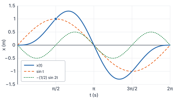
A 1 kg mass hangs on a spring with spring constant 4 N/m and no damping. It starts at rest at equilibrium, and an outside force of 3 sin t newtons acts on it. Its position x(t), in meters, satisfies x″ + 4x = 3 sin t, x(0) = 0, x′(0) = 0. Find x(t) and the position at t = π/2 seconds.
s^2X - 0 - 0 + 4X = \dfrac{3}{s^2 + 1}Transform both sides; L{sin t} = 1/(s² + 1).
(s^2 + 4)X = \dfrac{3}{s^2 + 1}Factor out X.
X = \dfrac{3}{(s^2 + 1)(s^2 + 4)}Divide by s² + 4.
\dfrac{3}{(s^2 + 1)(s^2 + 4)} = \dfrac{A}{s^2 + 1} + \dfrac{B}{s^2 + 4}Only s² appears, so use constant numerators.
3 = A(s^2 + 4) + B(s^2 + 1)
Clear denominators.
3 = 3A \Rightarrow A = 1
Substitute s² = −1.
3 = -3B \Rightarrow B = -1
Substitute s² = −4.
X = \dfrac{1}{s^2 + 1} - \dfrac{1}{2}\cdot\dfrac{2}{s^2 + 4}The sine row needs b = 2 on top, so multiply and divide by 2.
x(t) = \sin t - \tfrac{1}{2}\sin 2tInvert each piece.
x\left(\tfrac{\pi}{2}\right) = \sin\tfrac{\pi}{2} - \tfrac{1}{2}\sin\piSubstitute t = π/2.
x\left(\tfrac{\pi}{2}\right) = 1 - 0 = 1Use sin(π/2) = 1 and sin π = 0.
Answer: x(t) = sin t − (1/2) sin 2t meters, and the mass is 1 meter from equilibrium at t = π/2 seconds. The sin t part follows the outside force; the sin 2t part is the spring’s natural motion at ω = 2, as in spring-mass systems.
Example 5: A repeated root with exponential forcing
Solve y″ − 4y′ + 4y = 2e^(2t) with y(0) = 1 and y′(0) = 3.
s^2Y - s - 3 - 4(sY - 1) + 4Y = \dfrac{2}{s - 2}Transform both sides and substitute the initial values.
s^2Y - s - 3 - 4sY + 4 + 4Y = \dfrac{2}{s - 2}Distribute the −4.
(s^2 - 4s + 4)Y - s + 1 = \dfrac{2}{s - 2}Group the Y terms and combine −3 + 4.
(s - 2)^2Y = s - 1 + \dfrac{2}{s - 2}Factor the perfect square trinomial and add s − 1 to both sides.
Y = \dfrac{s - 1}{(s - 2)^2} + \dfrac{2}{(s - 2)^3}Divide both sides by (s − 2)².
s - 1 = (s - 2) + 1
Rewrite the numerator using s − 2.
Y = \dfrac{1}{s - 2} + \dfrac{1}{(s - 2)^2} + \dfrac{2}{(s - 2)^3}Split the first fraction.
\dfrac{2}{(s - 2)^3} = \dfrac{2!}{(s - 2)^{3}}Note 2! = 2, so this matches t²e^(2t).
y(t) = e^{2t} + te^{2t} + t^2e^{2t}Invert with the tⁿe^(at) row.
Answer: y(t) = e^(2t)(1 + t + t²). Check: y(0) = 1, and y′ = e^(2t)(3 + 4t + 2t²), so y′(0) = 3. The forcing e^(2t) matches the double root s = 2, so the transform produces the t²e^(2t) term without the guess-and-modify step of the method of undetermined coefficients.
Common mistakes
| Mistake | Example of the error | Fix |
|---|---|---|
| Wrong sign on the initial value | L{y′} = sY + y(0) | The rule is sY − y(0); initial values enter with minus signs. |
| Dropping the y′(0) term | L{y″} = s²Y − sy(0) | Write all three terms: s²Y − sy(0) − y′(0). |
| Not transforming a constant | y′ + 4y = 8 → sY − 1 + 4Y = 8 | A constant c transforms to c/s, so the right side is 8/s. |
| Multiplying only part of a rule by its coefficient | L{4y′} = 4sY − y(0) | Multiply the whole rule: 4(sY − y(0)). |
| Inverting a product directly | Y = (s + 8)/(s(s + 4)) → (1 + 8)e^(−4t) | Use partial fractions first, then invert each piece. |
| Adding C₁ and C₂ at the end | y = 2 − e^(−4t) + C | The initial conditions are already in Y(s); there are no constants left. |
Related methods
Laplace transforms vs. the characteristic equation
| Situation | Characteristic equation with undetermined coefficients | Laplace transform method |
|---|---|---|
| Homogeneous, constant coefficients | Fast: find the roots, then solve for C₁ and C₂ | Works; the denominator is the characteristic polynomial |
| Polynomial, exponential or sine forcing | Guess a particular solution, then fit the initial values | Handles the forcing and initial values in one pass |
| Piecewise or impulse forcing | Hard: solve on each interval and match | Natural fit (step and delta functions) |
| Variable coefficients or nonlinear | Use other methods | Usually does not apply |
Initial conditions at a time other than 0
The derivative rules use y(0) and y′(0). If the conditions are given at t = t₀, substitute τ = t − t₀, solve for y as a function of τ starting at τ = 0, and then replace τ with t − t₀.
Piecewise forcing
The method really pays off when the forcing switches on and off, like a voltage that turns on at t = 2. That needs the step function, covered next in Unit Step Functions. Forced springs without damping can also show resonance, which the transform handles with repeated factors.
Practice problems
- Solve y′ − 2y = 0 with y(0) = 5.
- Solve y′ + 3y = 6 with y(0) = 0.
- Solve y′ − y = e^(2t) with y(0) = 0.
- Solve y″ + 9y = 0 with y(0) = 2 and y′(0) = 6.
- Solve y″ − 3y′ + 2y = 0 with y(0) = 0 and y′(0) = 1.
- Solve y″ + 4y′ + 4y = 0 with y(0) = 1 and y′(0) = 0.
- Solve y″ + 4y′ + 13y = 0 with y(0) = 1 and y′(0) = 4.
- Solve y″ + y = 2 with y(0) = 0 and y′(0) = 0.
- Solve y″ − 4y = 8 with y(0) = 0 and y′(0) = 0.
- An RL circuit with inductance 0.5 H, resistance 10 Ω and a 20 V battery has current i(t), in amperes, with 0.5i′ + 10i = 20 and i(0) = 0. Find i(t) and the long-run current.
Show answers
1.
sY - 5 - 2Y = 0
Transform and substitute y(0) = 5.
(s - 2)Y = 5
Factor out Y and add 5 to both sides.
Y = \dfrac{5}{s - 2}Divide by s − 2.
Answer: y = 5e^(2t)
2.
sY - 0 + 3Y = \dfrac{6}{s}Transform and substitute y(0) = 0.
Y = \dfrac{6}{s(s + 3)}Factor out Y and divide by s + 3.
6 = A(s + 3) + Bs
Clear denominators in A/s + B/(s + 3).
A = 2,\quad B = -2
Substitute s = 0 (6 = 3A), then s = −3 (6 = −3B).
Y = \dfrac{2}{s} - \dfrac{2}{s + 3}Write the pieces.
Answer: y = 2 − 2e^(−3t)
3.
sY - 0 - Y = \dfrac{1}{s - 2}Transform and substitute y(0) = 0.
Y = \dfrac{1}{(s - 1)(s - 2)}Factor out Y and divide by s − 1.
1 = A(s - 2) + B(s - 1)
Clear denominators in A/(s − 1) + B/(s − 2).
A = -1,\quad B = 1
Substitute s = 1 (1 = −A), then s = 2 (1 = B).
Y = \dfrac{1}{s - 2} - \dfrac{1}{s - 1}Write the pieces.
Answer: y = e^(2t) − e^t
4.
s^2Y - 2s - 6 + 9Y = 0
Transform and substitute y(0) = 2 and y′(0) = 6.
Y = \dfrac{2s + 6}{s^2 + 9}Factor out Y, add 2s + 6 to both sides and divide.
Y = 2\cdot\dfrac{s}{s^2 + 9} + 2\cdot\dfrac{3}{s^2 + 9}Split, writing 6 as 2 · 3 for the sine row with b = 3.
Answer: y = 2 cos 3t + 2 sin 3t
5.
s^2Y - 0 - 1 - 3(sY - 0) + 2Y = 0
Transform and substitute y(0) = 0 and y′(0) = 1.
(s^2 - 3s + 2)Y = 1
Group the Y terms and add 1 to both sides.
Y = \dfrac{1}{(s - 1)(s - 2)}Factor and divide.
Y = \dfrac{1}{s - 2} - \dfrac{1}{s - 1}Same partial fractions as problem 3.
Answer: y = e^(2t) − e^t
6.
s^2Y - s - 0 + 4(sY - 1) + 4Y = 0
Transform and substitute y(0) = 1 and y′(0) = 0.
(s^2 + 4s + 4)Y = s + 4
Group the Y terms and move −s − 4 to the right side.
Y = \dfrac{s + 4}{(s + 2)^2}Factor the perfect square and divide.
s + 4 = (s + 2) + 2
Rewrite the numerator using s + 2.
Y = \dfrac{1}{s + 2} + \dfrac{2}{(s + 2)^2}Split the fraction.
Answer: y = e^(−2t) + 2te^(−2t)
7.
s^2Y - s - 4 + 4(sY - 1) + 13Y = 0
Transform and substitute y(0) = 1 and y′(0) = 4.
(s^2 + 4s + 13)Y = s + 8
Group the Y terms and move −s − 8 to the right side.
s^2 + 4s + 13 = (s + 2)^2 + 9
Complete the square.
s + 8 = (s + 2) + 6
Rewrite the numerator using s + 2.
Y = \dfrac{s + 2}{(s + 2)^2 + 9} + 2\cdot\dfrac{3}{(s + 2)^2 + 9}Split, writing 6 as 2 · 3 for b = 3.
Answer: y = e^(−2t)cos 3t + 2e^(−2t)sin 3t
8.
s^2Y - 0 - 0 + Y = \dfrac{2}{s}Transform and substitute the zero initial values.
Y = \dfrac{2}{s(s^2 + 1)}Factor out Y and divide by s² + 1.
2 = A(s^2 + 1) + (Bs + C)s
Clear denominators in A/s + (Bs + C)/(s² + 1).
A = 2
Substitute s = 0.
0 = (2 + B)s^2 + Cs \Rightarrow B = -2,\ C = 0
Subtract 2 and match coefficients.
Y = \dfrac{2}{s} - \dfrac{2s}{s^2 + 1}Write the pieces.
Answer: y = 2 − 2 cos t
9.
s^2Y - 0 - 0 - 4Y = \dfrac{8}{s}Transform and substitute the zero initial values.
Y = \dfrac{8}{s(s - 2)(s + 2)}Factor out Y and divide by s² − 4 = (s − 2)(s + 2).
8 = A(s - 2)(s + 2) + Bs(s + 2) + Cs(s - 2)
Clear denominators in A/s + B/(s − 2) + C/(s + 2).
A = -2
Substitute s = 0: 8 = −4A.
B = 1
Substitute s = 2: 8 = 8B.
C = 1
Substitute s = −2: 8 = 8C.
Answer: y = −2 + e^(2t) + e^(−2t)
10.
i' + 20i = 40
Multiply both sides by 2.
sI - 0 + 20I = \dfrac{40}{s}Transform and substitute i(0) = 0.
I = \dfrac{40}{s(s + 20)}Factor out I and divide by s + 20.
40 = A(s + 20) + Bs
Clear denominators in A/s + B/(s + 20).
A = 2,\quad B = -2
Substitute s = 0 (40 = 20A), then s = −20 (40 = −20B).
I = \dfrac{2}{s} - \dfrac{2}{s + 20}Write the pieces.
Answer: i(t) = 2 − 2e^(−20t) amperes; as t grows, e^(−20t) goes to 0, so the long-run current is 2 A (which is 20 V ÷ 10 Ω).
Solving differential equations with Laplace transforms FAQ
Why use Laplace transforms to solve differential equations?
The transform turns a linear differential equation into an algebra equation and builds in the initial conditions. It is especially useful when the forcing is piecewise or an impulse, where other methods get messy.
What is the Laplace transform of y″?
It is L{y″} = s²Y(s) − sy(0) − y′(0). For the first derivative, L{y′} = sY(s) − y(0).
Can Laplace transforms solve nonlinear differential equations?
Usually not. The method relies on linearity, so a term like y² or sin y has no simple transform in terms of Y(s). It also gets hard when the coefficients depend on t.
What if the initial conditions are not at t = 0?
Shift time with τ = t − t₀ so the conditions are at τ = 0. Solve in τ with the usual rules, then replace τ with t − t₀.
Summary
- Transform both sides, using L{y′} = sY − y(0) and L{y″} = s²Y − sy(0) − y′(0).
- Substitute the initial conditions right away, then solve the algebra equation for Y(s).
- The coefficient of Y(s) is the characteristic polynomial of the equation.
- Use partial fractions or completing the square, then invert each piece to get y(t).
- No constants are left at the end; check the answer in the equation and the initial conditions.
Previous lesson: Inverse Laplace Transform
Next lesson: Unit Step Functions
Back to the Differential Equations Index